|
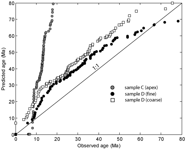
The gray circles on Figure 6 show the observed CAD of
sample C (sand collected at the apex of the alluvial fan). The
difference with the predicted CAD is immediately apparent. A useful
tool for comparing two (cumulative) distributions is the
quantile-quantile (Q-Q) plot [p. 353 of Rice, 1995]. In a Q-Q
plot, the quantiles of one distribution are plotted against those of
another. Two distributions are equal if and only if they plot on the
1:1-line. This is clearly not the case for the CAD of sample C (gray
circles on Figure 7). Sample C consists of very young
ages between 6 and 19Ma indicating that it was derived from very low
elevations. This very localized provenance of sample C suggests that
sediments in the presently active Marble Creek are derived from a
single rock fall event localized very close to the mouth of the Marble
Creek drainage, at an elevation of at most 500m above the sample
location (Figures 1 and 2).

|
Thus far, we have studied clasts A and B and a single sand sample C.
The next logical study is a composite of the entire alluvial fan, in
an attempt to get a more integrated view of the entire drainage basin.
47 samples were collected from all over the alluvial fan (sample D:
circles on Figure 2). These samples can be jointly
considered, because the time span covered by fan surfaces in debris
flow dominated alluvial fans of the Owens Valley is relatively short
(![]() 100ka; Dühnforth et al., 2007). To estimate the
possible importance of grain-size induced bias, these samples were
divided into a coarse (5 cm
100ka; Dühnforth et al., 2007). To estimate the
possible importance of grain-size induced bias, these samples were
divided into a coarse (5 cm ![]() clasts
clasts ![]() 7.925 mm) and a fine (2.794
mm
7.925 mm) and a fine (2.794
mm ![]() clasts
clasts ![]() 0.595 mm) fraction. Then, the samples from each of
the two groups were mixed and dated with the AFT method. The
resulting CADs are shown as white squares and black circles on Figure
6. Most apatites in the composite sample are older
than sample C. The coarse fraction appears to be slightly younger
than the fine fraction, but the difference is not statistically
significant (compare the distance between the two CADs with the width
of the gray confidence band in Figure 6), and we may
conclude that grain-size effects are not very important. Just as we
did for sample C, we compare the observed and predicted CADs for
sample D by plotting them on a Q-Q plot (Figure 7).
This analysis indicates that the composite sample was derived from the
entire drainage. Most of the sediment was derived from low
elevations, with smaller contributions from further away.
0.595 mm) fraction. Then, the samples from each of
the two groups were mixed and dated with the AFT method. The
resulting CADs are shown as white squares and black circles on Figure
6. Most apatites in the composite sample are older
than sample C. The coarse fraction appears to be slightly younger
than the fine fraction, but the difference is not statistically
significant (compare the distance between the two CADs with the width
of the gray confidence band in Figure 6), and we may
conclude that grain-size effects are not very important. Just as we
did for sample C, we compare the observed and predicted CADs for
sample D by plotting them on a Q-Q plot (Figure 7).
This analysis indicates that the composite sample was derived from the
entire drainage. Most of the sediment was derived from low
elevations, with smaller contributions from further away.
![]() 5% of the detrital grains in sample D have a zero AFT age
whereas other apatites appear to be well over 100 Ma old, apparently
contradicting the 10-55 Ma age range predicted by the PAZ-curve of
Stockli et al. [2000]. At first glance, this observation seems
to suggest that some apatites are derived from outside the Marble
Creek catchment. There are at least two possible sources for such
``contamination'': (1) the catchment is down wind from the Long Valley
caldera, and the area was likely covered by a thick layer of Bishop
volcanic ash; and (2) eolian processes in the arid Owens Valley might
contaminate the Marble Creek alluvial fan with modern dust. The first
possibility can be ruled out because the relatively coarse grain-size
of sample D allowed verification of its granite and marble
composition. Virtually no tuff was found. The coarse grain-size of
sample D also drastically reduces the probability of modern eolian
contamination. Alternatively, the ``anomalous'' AFT ages can be much
more easily explained by the counting statistics discussed in Section
2.
5% of the detrital grains in sample D have a zero AFT age
whereas other apatites appear to be well over 100 Ma old, apparently
contradicting the 10-55 Ma age range predicted by the PAZ-curve of
Stockli et al. [2000]. At first glance, this observation seems
to suggest that some apatites are derived from outside the Marble
Creek catchment. There are at least two possible sources for such
``contamination'': (1) the catchment is down wind from the Long Valley
caldera, and the area was likely covered by a thick layer of Bishop
volcanic ash; and (2) eolian processes in the arid Owens Valley might
contaminate the Marble Creek alluvial fan with modern dust. The first
possibility can be ruled out because the relatively coarse grain-size
of sample D allowed verification of its granite and marble
composition. Virtually no tuff was found. The coarse grain-size of
sample D also drastically reduces the probability of modern eolian
contamination. Alternatively, the ``anomalous'' AFT ages can be much
more easily explained by the counting statistics discussed in Section
2.