Introduction

Radiometric cooling ages ($^{40}$Ar/$^{39}$Ar, fission track, (U-Th)/He) of exhumed fault blocks generally increase with elevation. For catchments draining such terranes, it is possible to predict detrital age distributions if the relationship between age and elevation is either assumed or known, if the catchment hypsometry is known, and under some additional assumptions, which are discussed below.

A few studies have explored this for the $^{40}$Ar/$^{39}$Ar system. If erosion is in a steady state over geologic time, then $^{40}$Ar/$^{39}$Ar cooling ages are expected to decrease linearly with depth, or increase linearly with elevation. In a theoretical study, Stock and Montgomery [1996] argue that, under the assumption of a thermal gradient, the range of detrital cooling ages can be used to estimate (paleo-)relief. Going one step further, Brewer et al. (2003) proposed a method to estimate average basin-wide erosion rates by matching the shape of detrital age distributions with the area-elevation curve (= ``hypsometry'') of the catchment. In a recent paper, Ruhl and Hodges [2005] introduced a hybrid approach using an extensive dataset of 692 detrital muscovite $^{40}$Ar/$^{39}$Ar ages from four catchments in the Himalaya. Average basin-wide erosion rates were estimated from the range of detrital cooling ages, while the shape of the detrital age distributions was used to test the validity of several assumptions made by Stock and Montgomery [1996] and Brewer et al. [2003]: (1) the assumption of steady-state erosion and topography, which is required for a predictable (typically linear) age-elevation curve, and (2) the assumptions of uniform modern erosion rates, negligible sediment storage in the catchment and adequate mixing of the sediments, which are necessary for the convolution of this age-elevation curve with the catchment hypsometry, but may be invalidated by inhomogeneous lithologies, structural geology or the presence or absence of vegetation.

If these assumptions hold, Ruhl and Hodges [2005] argue, then the hypsometric curve must match the observed detrital age distribution. Strictly speaking, this does not mean that all assumptions hold if and only if the hypsometry matches the measured detrital age distribution. More importantly, if the measured age distribution does not match the hypsometry, it is difficult to assess which of the assumptions were violated and to what extent. In only one of Ruhl and Hodges' [2005] four catchments did the measured match the predicted age distribution, indicating that steady-state erosion might exist. For the other three catchments, it is unclear whether this means that erosion and topography are not in steady-state, erosion rates are not uniform or sediments are not well mixed. Is one problem responsible for all catchments or are different assumptions violated in different catchments? For each of the previous studies, the age-elevation relationship was unkown. If known, would that have explained the mismatches that resulted from assuming a linear age-elevation relation? The present paper avoids many of these questions in a carefully selected field area, where assumption 1 is not necessary, enabling a semi-quantitative assessment of assumption 2. The following sections will outline a method to map out the erosion rate distribution in a watershed by looking at the frequency distribution of detrital fission track cooling ages in apatite crystals derived from it. This idea was independently developed and published by Stock et al. [2006], who studied detrital (U-Th)/He ages from two catchments in the eastern Sierra Nevada, on the opposite side of the Owens Valley. Although the basic idea behind the work of Stock et al. [2006] is identical to the present study, there are important methodological differences in the way the data are interpreted (Section 2).

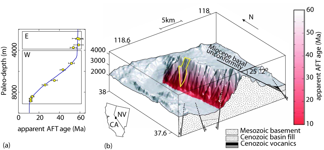
The method is illustrated in the context of a simple drainage basin in the White Mountains, an eastward-tilted fault block on the California-Nevada border. The S-N trending White Mountains fault block is bounded on the west by the White Mountains fault zone, which is dated at 12 Ma by AFT and (U-Th)/He dating at different structural levels on the fault block [Stockli et al., 2000, 2003]. A mid-Miocene erosional unconformity found on the eastern flank of the northern White Mountains is tilted $\sim$ 25$^o$ to the east [ Stockli et al., 2000, 2003]. Linearly extrapolating this Miocene paleo-surface would imply up to 8 km of normal displacement along the White Mountains fault zone. The eastern boundary of the White Mountains is marked by the dextral Fish Lake fault zone, which initiated at 6 Ma, and corresponds to the onset of strike-slip motion on the Walker Lane Belt [Stewart, 1988; Reheis and Dixon, 1996; Reheis and Sawyer, 1997]. At 3 Ma, the White Mountains fault zone was reactivated in an oblique right-lateral strike-slip sense, marking the progression of Walker Lane tectonism from east to west [Stockli et al., 2003]. The dip-slip component of motion was large enough that its signal can be recognized in the exhumed (U-Th)/He Partial Retention Zone (PRZ) of the northern White Mountains [Stockli et al., 2000, 2003].

Figure 1: (a) The AFT data of Stockli et al. [2000] reveal an exhumed Partial Annealing Zone (PAZ). Each paleodepth under a Miocene erosional unconformity corresponds to a unique AFT age. The lower part of this curve is exposed on the western side of the range (box labeled ``W''), whereas the upper part is exposed on the eastern side (box labeled ``E''). (b) For each location on the northern White Mountains, the paleodepth was calculated, and using (a), the corresponding AFT age was computed, and color-coded. The yellow polygon outlines the Marble Creek drainage basin.

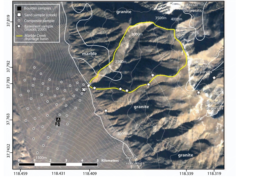
Stockli et al. [2000] measured AFT and apatite (U-Th)/He ages along a transect in the northern White Mountains (Figures 1 and 2), revealing an exhumed fission track Partial Annealing Zone (PAZ, Figure 1.a). Defining ``paleodepth'' as the perpendicular distance to the assumed tilted mid-Miocene erosional surface, each paleodepth in Figure 1.a corresponds to a unique AFT age and conversely, each AFT age corresponds to a unique paleodepth. AFT ages can be predicted by computing the paleodepth for each pixel of a digital elevation model (DEM), and assigning the corresponding AFT age to it. This is exactly how Figure 1.b was generated. The paleodepth values of Stockli et al. [2000] are based on the interpretation that a bedding dip in the eastern White Mountains could be reliably projected across the range into space (Figure 1.b). It is, however, possible that this surface was folded, potentially causing significant uncertainties on the paleodepths. This would have little or no effect on the reconstructed AFT age-distribution. Paleodepth is just used as an intermediate step between AFT age and topography. Exactly via which numerical paleodepth-value an AFT age is mapped to a topographic location is irrelevant, as long as the mapping is correct.

If we assume that the sand grains were uniformly derived from the entire drainage (assumption 2 of Ruhl and Hodges, 2005), it is possible to predict the detrital AFT grain-age distribution. Detrital thermochronological data are usually represented by estimates of their probability density, whose interpretation often involves deconvolution into Gaussian subpopulations [Galbraith and Green, 1990; Brandon, 1996]. Cumulative distributions are an alternative to probability density estimates that have recently gained considerable popularity [Brewer et al, 2003; Amidon et al., 2005; Ruhl and Hodges, 2005; Hodges et al., 2005]. This paper introduces a new kind of cumulative distribution which is slightly different from these previous studies. The reasons why this so-called ``Cumulative Age Distribution'' is preferred to probability density estimates and previous cumulative probability curves are discussed in the following section.

Figure 2: Landsat image of the Marble Creek drainage basin and its alluvial fan, with indication of the sample locations and the underlying geology, modified from Saucedo et al. [2000] and McKee and Conrad [1996].