Before calculating an exposure age or erosion rate, it is a good idea
to check if the TCN measurements are consistent with a simple or
complex exposure history. This can be done with two nuclides
(including at least one radionuclide) using a ``banana plot'' (Lal,
1991). CosmoCalc accomodates two types of banana plot:
![]() Al-
Al-![]() Be and
Be and ![]() Ne-
Ne-![]() Be. Depending on whether or
not a sample plots above, below or inside the so-called ``steady-state
erosion island'' (Lal, 1991), one can decide whether or not to pursue
the calculation of an exposure age, erosion rate or burial age. For
the construction of the banana plots and the age/erosion calculations
of Section 5, CosmoCalc implements a modified version of
the ingrowth equation of Granger and Muzikar (2001):
Be. Depending on whether or
not a sample plots above, below or inside the so-called ``steady-state
erosion island'' (Lal, 1991), one can decide whether or not to pursue
the calculation of an exposure age, erosion rate or burial age. For
the construction of the banana plots and the age/erosion calculations
of Section 5, CosmoCalc implements a modified version of
the ingrowth equation of Granger and Muzikar (2001):
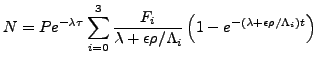
With N the nuclide concentration (atoms/g), P the total surface
production rate (in atoms/g/yr) at SLHL, ![]() the burial age,
the burial age,
![]() the erosion rate, t the exposure age and
the erosion rate, t the exposure age and ![]() the
radioactive half-life of the nuclide. Equation 4
models TCN production by neutrons, slow and fast muons by a series of
exponential approximations. The first term of the summation models
TCN production by spallogenic neutron reactions, the second and third
terms model slow muons and the last term approximates TCN production
by fast muons. Thus,
the
radioactive half-life of the nuclide. Equation 4
models TCN production by neutrons, slow and fast muons by a series of
exponential approximations. The first term of the summation models
TCN production by spallogenic neutron reactions, the second and third
terms model slow muons and the last term approximates TCN production
by fast muons. Thus,
![]() are dimensionless numbers between
zero and one, and
are dimensionless numbers between
zero and one, and
![]() are attenuation lengths
(g/cm
are attenuation lengths
(g/cm![]() ). The approach of Granger et al. (2000, 2001) was chosen
because of its flexibility. For instance, neglecting muon production
can be easily implemented by setting
). The approach of Granger et al. (2000, 2001) was chosen
because of its flexibility. For instance, neglecting muon production
can be easily implemented by setting ![]() and
and ![]() equal to zero
in Equation 4. CosmoCalc uses Granger et al.'s (2000,
2001) recommended values of
equal to zero
in Equation 4. CosmoCalc uses Granger et al.'s (2000,
2001) recommended values of
![]() for
for ![]() Be and
Be and ![]() Al,
but also offers an alternative choice of pre-set values approximating
either the alternative parameterization of Schaller et al. (2001),
neglecting the contribution of muons, or only using three exponentials
(for more details, see Section 7). Banana plots with
non-zero muon contributions feature a characteristic cross-over of the
steady-state and zero erosion lines which is absent when muons are
neglected (Figure 2).
Al,
but also offers an alternative choice of pre-set values approximating
either the alternative parameterization of Schaller et al. (2001),
neglecting the contribution of muons, or only using three exponentials
(for more details, see Section 7). Banana plots with
non-zero muon contributions feature a characteristic cross-over of the
steady-state and zero erosion lines which is absent when muons are
neglected (Figure 2).
CosmoCalc's banana plots are normalized to SLHL, meaning that the TCN
concentrations of each sample are divided by the cumulative effect of
all their correction factors, represented by the ``effective scaling
factor'' ![]() :
:
with
where ![]() is one of the production rate scaling factors of Section
2 and
is one of the production rate scaling factors of Section
2 and ![]() ,
, ![]() and
and ![]() are defined in Section
3. If muon production is neglected, then
are defined in Section
3. If muon production is neglected, then ![]() =
=
![]() . However, in the presence of
muons, the effective scaling factor
. However, in the presence of
muons, the effective scaling factor ![]() may deviate from this value
because the relative importance of the different production mechanisms
changes as a function of age, erosion rate, elevation, latitude,
sample thickness and snow cover. The exact form of the function f(S)
will be defined in Section 5. Note that the topographic
shielding correction
may deviate from this value
because the relative importance of the different production mechanisms
changes as a function of age, erosion rate, elevation, latitude,
sample thickness and snow cover. The exact form of the function f(S)
will be defined in Section 5. Note that the topographic
shielding correction ![]() does not ``fractionate'' (i.e., change the
fractions
does not ``fractionate'' (i.e., change the
fractions ![]() ,...,
,...,![]() of) the different production mechanisms and
is placed outside the scaling function f(S). This means that,
strictly speaking, the TCN concentrations should be multiplied by
of) the different production mechanisms and
is placed outside the scaling function f(S). This means that,
strictly speaking, the TCN concentrations should be multiplied by
![]() prior to generating a banana plot. The input required by
CosmoCalc's ``Banana'' function are (1) the composite scaling factor S
for the first nuclide (
prior to generating a banana plot. The input required by
CosmoCalc's ``Banana'' function are (1) the composite scaling factor S
for the first nuclide (![]() Al or
Al or ![]() Ne), (2) the concentration
and 1
Ne), (2) the concentration
and 1![]() measurement uncertainty of the first nuclide (
measurement uncertainty of the first nuclide (![]() Al
or
Al
or ![]() Ne), both multiplied by
Ne), both multiplied by ![]() , (3) S for the second nuclide
(
, (3) S for the second nuclide
(![]() Be) and (4) the concentration and 1
Be) and (4) the concentration and 1![]() measurement
uncertainty of the second nuclide (
measurement
uncertainty of the second nuclide (![]() Be), also multiplied by
Be), also multiplied by
![]() . Because topographic shielding corrections are generally small,
the systematic error caused by lumping
. Because topographic shielding corrections are generally small,
the systematic error caused by lumping ![]() together with the other
correction factors is very small. Therefore, if
together with the other
correction factors is very small. Therefore, if
![]() 0.95,
say, it is safe to approximate Equation 5 by
0.95,
say, it is safe to approximate Equation 5 by ![]() = f(
= f(
![]() ). In this case, the nuclide
concentrations do not need to be pre-multiplied by
). In this case, the nuclide
concentrations do not need to be pre-multiplied by ![]() .
.
|
a. 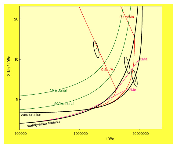
b. 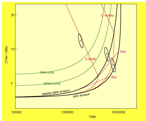 |
The graphical output of CosmoCalc can easily be copied and pasted for
editing in vector graphics software such as Adobe Illustrator or
CorelDraw. The y-axis of the ![]() Al-
Al-![]() Be plot is logarithmic
by default whereas the y-axis of the
Be plot is logarithmic
by default whereas the y-axis of the ![]() Ne-
Ne-![]() Be plot is
linear. These defaults can be changed in the ``Banana Options''
userform. Note that MS-Excel (versions 2000 and 2003) only allows
logarithmic tickmarks to have values in multiples of ten. To get
around this limitation, CosmoCalc uses a ``pseudo y-axis'', which
cannot be edited by the usual right mousebutton-click. Hopefully,
this limitation will not be necessary in later versions of Excel.
CosmoCalc only propagates the analytical uncertainty of the measured
TCN concentrations. No uncertainty is assigned to the production rate
scaling factors, radioactive half-lives or other potentially
ill-constrained quantities. On the banana plots, the user is offered
the choice between error bars or -ellipses with the latter being the
default. Banana plots are graphs of the type
Be plot is
linear. These defaults can be changed in the ``Banana Options''
userform. Note that MS-Excel (versions 2000 and 2003) only allows
logarithmic tickmarks to have values in multiples of ten. To get
around this limitation, CosmoCalc uses a ``pseudo y-axis'', which
cannot be edited by the usual right mousebutton-click. Hopefully,
this limitation will not be necessary in later versions of Excel.
CosmoCalc only propagates the analytical uncertainty of the measured
TCN concentrations. No uncertainty is assigned to the production rate
scaling factors, radioactive half-lives or other potentially
ill-constrained quantities. On the banana plots, the user is offered
the choice between error bars or -ellipses with the latter being the
default. Banana plots are graphs of the type ![]() /
/![]() vs.
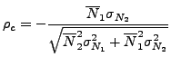
vs. ![]() which are always associated with some degree of ``spurious
correlation'' (Chayes, 1949). This causes the error ellipses to be
rotated according to the following correlation coefficient:
which are always associated with some degree of ``spurious
correlation'' (Chayes, 1949). This causes the error ellipses to be
rotated according to the following correlation coefficient:
If ![]() stands for
stands for ![]() Al or
Al or ![]() Ne and
Ne and ![]() for
for ![]() Be,
then
Be,
then
![]() and
and
![]() are the measured
concentrations of these respective nuclides while
are the measured
concentrations of these respective nuclides while
![]() and
and
![]() are the corresponding measurement uncertainties.
are the corresponding measurement uncertainties.