Customizing CosmoCalc

The interface of CosmoCalc is very simple because default values are set for most of the parameters that occur in the various equations discussed in this paper (Table 1). This greatly reduces the chance that novice users make mistakes when reducing their TCN data. For more advanced users, the program allows nearly all the parameters to be changed.

Specifying the production rate calibration sites

As mentioned in Section 2, it is very important to use a consistent set of scaling factors for the unknown sample and the production rate calibration site. Failing to do so can cause significant systematic errors. To avoid this, CosmoCalc defines the SLHL production rates implicitly, by specifying a set of calibration sites and their measured TCN concentrations. Using the ``Calibration sites'' form of the ``Settings'' menu, these concentrations are scaled to SLHL and an average production rate is calculated using one of the five scaling models of Section 2. CosmoCalc comes with a default set of published production rate calibrations, some of which ($^{10}$Be and $^{26}$Al) were borrowed from Balco and Stone (2007; http://hess.ess.washington.edu/math). The published data come from a variety of latitudes and elevations, yielding a presumably reliable estimate of the globally averaged production rates. This, however, is not always the best approach. For example, if a TCN study is carried out in the vicinity of one particular calibration site, then it makes more sense to use only this site to estimate the local production rate. Therefore, CosmoCalc offers the user the flexibility to delete or add calibration sites at will.

Changing the relative contributions of different production pathways

Being based on the equation of Granger and Smith (2000), the TCN production equation consists of four exponentials: one for neutrons, two for slow neutrons, and one for fast neutrons (see Equation 8 and Section 5). These exponentials are governed by two sets of parameters: the fractions $F_i$ and the attenuation lengths $\Lambda_i$ (for i=0,...,3). Default values for $\Lambda_i$, $F_i$($^{10}$Be) and $F_i$($^{26}$Al) were taken from Granger and Smith (2000) (Table 1), but these values can be changed in the ``Settings'' form.

Table 1: Default values of CosmoCalc parameters

parameter	symbol	default value	units
rock density	$\rho$	2.65	g/cm$^3$
decay constant ($^{10}$Be)	$\lambda$($^{10}$Be)	4.560E-07	yr$^{-1}$
decay constant ($^{26}$Al)	$\lambda$($^{26}$Al)	9.800E-07	yr$^{-1}$
decay constant ($^{36}$Cl)	$\lambda$($^{36}$Cl)	2.300E-06	yr$^{-1}$
decay constant ($^{14}$C)	$\lambda$($^{14}$C)	1.213E-04	yr$^{-1}$
attenuation length (neutrons)	$\Lambda_0$	160	g/cm$^2$
attenuation length (slow muons)	$\Lambda_1$	738	g/cm$^2$
attenuation length (slow muons)	$\Lambda_2$	2688	g/cm$^2$
attenuation length (fast muons)	$\Lambda_3$	4360	g/cm$^2$
relative production by neutrons ($^{10}$Be)	$F_0$($^{10}$Be)	0.9724	-
relative production by neutrons ($^{26}$Al)	$F_0$($^{26}$Al)	0.9655	-
relative production by neutrons ($^{14}$C)	$F_0$($^{14}$C)	0.83	-
relative production by neutrons ($^{36}$Cl)	$F_0$($^{36}$Cl)	0.903	-
relative production by neutrons ($^{3}$He)	$F_0$($^{3}$He)	1	-
relative production by neutrons ($^{21}$Ne)	$F_0$($^{21}$Ne)	1	-
relative production by slow muons ($^{10}$Be)	$F_1$($^{10}$Be)	0.0186	-
relative production by slow muons ($^{26}$Al)	$F_1$($^{26}$Al)	0.0233	-
relative production by slow muons ($^{14}$C)	$F_1$($^{14}$C)	0.0691	-
relative production by slow muons ($^{36}$Cl)	$F_1$($^{36}$Cl)	0.0447	-
relative production by slow muons ($^{3}$He)	$F_1$($^{3}$He)	0	-
relative production by slow muons ($^{21}$Ne)	$F_1$($^{21}$Ne)	0	-
relative production by slow muons ($^{10}$Be)	$F_2$($^{10}$Be)	0.004	-
relative production by slow muons ($^{26}$Al)	$F_2$($^{26}$Al)	0.005	-
relative production by slow muons ($^{14}$C)	$F_2$($^{14}$C)	0.0809	-
relative production by slow muons ($^{36}$Cl)	$F_2$($^{36}$Cl)	0.0523	-
relative production by slow muons ($^{3}$He)	$F_2$($^{3}$He)	0	-
relative production by slow muons ($^{21}$Ne)	$F_2$($^{21}$Ne)	0	-
relative production by fast muons ($^{10}$Be)	$F_3$($^{10}$Be)	0.005	-
relative production by fast muons ($^{26}$Al)	$F_3$($^{26}$Al)	0.0062	-
relative production by fast muons ($^{14}$C)	$F_3$($^{14}$C)	0.02	-
relative production by fast muons ($^{36}$Cl)	$F_3$($^{36}$Cl)	0	-
relative production by fast muons ($^{3}$He)	$F_3$($^{3}$He)	0	-
relative production by fast muons ($^{21}$Ne)	$F_3$($^{21}$Ne)	0	-
sea level temperature	$T_0$	288.15	K
adiabatic lapse rate	$\beta_0$	6.5	K/km
air pressure at sea level	$p_0$	1013.25	mbar
geomagnetic field intensity relative to 1945	M/$M_0$	1	-

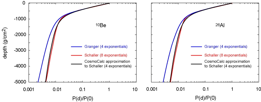
In addition to Equation 8, several alternative, but similar looking TCN ingrowth equations exist in the literature. Schaller et al. (2001, 2002) use not four but eight exponentials (two for neutrons, and three for each slow and fast muons), whereas others use three (one for each production mechanism) (e.g., Braucher et al., 2003; Miller et al., 2006) or only one exponential (neglecting muon production). CosmoCalc provides a separate set of default parameters for each of these alternatives. For example, the ingrowth equation of Schaller et al. (2002) was recast in the parameterization of Granger and Smith (2000) by a least squares fit of a virtual depth profile (Figure 4).

Figure 4: To implement the TCN ingrowth equation of Schaller et al. (2001, 2002), CosmoCalc uses a least squares fit of the TCN ingrowth equation of Granger and Smith (2000) to a ``virtual'' depth profile defined by this alternative ingrowth equation.