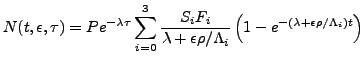
Equation 4 has three unknowns: t (exposure age),
![]() (erosion rate) and
(erosion rate) and ![]() (burial age). If only one nuclide
was measured, we must assume values for two of these quantities in
order to solve for the third. If two nuclides were analysed (of which
at least one is radioactive), only one assumption is needed.
CosmoCalc is capable of both approaches. In this section, we will
first discuss how to solve for
(burial age). If only one nuclide
was measured, we must assume values for two of these quantities in
order to solve for the third. If two nuclides were analysed (of which
at least one is radioactive), only one assumption is needed.
CosmoCalc is capable of both approaches. In this section, we will
first discuss how to solve for ![]() (assuming infinite exposure
age and zero burial) and t (assuming zero erosion and burial) using a
single nuclide (Section 5). Then, numerical methods will
be presented to simultaneously solve for t and
(assuming infinite exposure
age and zero burial) and t (assuming zero erosion and burial) using a
single nuclide (Section 5). Then, numerical methods will
be presented to simultaneously solve for t and ![]() (assuming
zero burial), t and
(assuming
zero burial), t and ![]() (assuming zero erosion) or
(assuming zero erosion) or ![]() and
and
![]() (assuming infinite exposure age), using two nuclides (Section
5). Note that in the case of two nuclides (
(assuming infinite exposure age), using two nuclides (Section
5). Note that in the case of two nuclides (![]() Al or
Al or
![]() Ne combined with
Ne combined with ![]() Be), the assumption of zero burial can
be verified on the banana plot.
Be), the assumption of zero burial can
be verified on the banana plot.
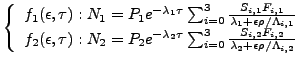
Calculations using a single nuclide
CosmoCalc requires three pieces of information to calculate an exposure age or erosion rate: the TCN concentration (corrected for topography), its analytical uncertainty and a composite correction factor for production rate scaling with latitude/elevation and shielding (Equation 6). We somehow need to incorporate this scaling factor into the ingrowth equation (Equation 4). This poses a problem because the scaling factor is a single number whereas Equation 4 explicitly makes the distinction between neutrons, slow and fast muons. Granger and Smith (2000) avoid this problem by separately scaling the different production mechanisms:
Instead of one scaling factor, Equation 8 has four, one
for neutrons (![]() ), two for slow muons (
), two for slow muons (![]() and
and ![]() ) and one for
fast muons (
) and one for
fast muons (![]() ). Granger et al. (2001) separately calculate each of
these four scaling factors. Thus, the original method of Granger and
Smith (2000) is incompatible with the common practice of lumping all
production mechanisms into a single latitude/elevation scaling factor
(Section 2). To ensure optimal flexibility and
user-friendliness, CosmoCalc uses a slightly different approach.
). Granger et al. (2001) separately calculate each of
these four scaling factors. Thus, the original method of Granger and
Smith (2000) is incompatible with the common practice of lumping all
production mechanisms into a single latitude/elevation scaling factor
(Section 2). To ensure optimal flexibility and
user-friendliness, CosmoCalc uses a slightly different approach.
![]() are calculated from the composite correction factor S,
by approximating the total scaling by a single attenuation factor
caused by a virtual layer of matter of thickness x (in g/cm
are calculated from the composite correction factor S,
by approximating the total scaling by a single attenuation factor
caused by a virtual layer of matter of thickness x (in g/cm![]() ):
):
so that
with ![]() and
and ![]() as in Equation 4 and S as
defined in Equation 6. CosmoCalc solves Equation 10
iteratively using Newton's method.
as in Equation 4 and S as
defined in Equation 6. CosmoCalc solves Equation 10
iteratively using Newton's method.
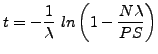
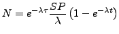
As said before, some assumptions are needed to solve Equation
8. An exposure age (t) can be calculated under the
assumption of zero erosion and burial (![]() = 0,
= 0, ![]() = 0).
For a radionuclide with decay constant
= 0).
For a radionuclide with decay constant ![]() , this yields:
, this yields:
whereas for stable nuclides (![]() He and
He and ![]() Ne):
Ne):
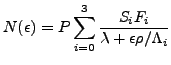
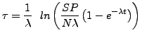
Alternatively, the erosion rate (![]() ) can be calculated under
the assumption of steady state and zero burial (t =
) can be calculated under
the assumption of steady state and zero burial (t = ![]() ,
,
![]() =0):
=0):
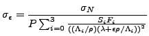
CosmoCalc solves this equation iteratively using Newton's method. Statistical uncertainties are estimated by standard error propagation:
These error estimates do not include any uncertainties in production rates and scaling factors, which are difficult to quantify, but can be evaluated by using a range of input parameters.
Calculations with two nuclides
Equation 8 has three unknowns (t, ![]() and
and ![]() ).
If two nuclides have been measured (with concentrations
).
If two nuclides have been measured (with concentrations ![]() and
and
![]() , say), only one value must be assumed in order to solve for the
remaining two. By assuming zero erosion (
, say), only one value must be assumed in order to solve for the
remaining two. By assuming zero erosion (![]() = 0), CosmoCalc
simultaneously calculates the exposure age and burial age (Section
5); by assuming steady-state erosion (t =
= 0), CosmoCalc
simultaneously calculates the exposure age and burial age (Section
5); by assuming steady-state erosion (t = ![]() ),
the erosion rate and burial age are calculated; and by assuming
zero-burial (
),
the erosion rate and burial age are calculated; and by assuming
zero-burial (![]() = 0), the erosion rate and exposure age can be
computed (Section 5).
= 0), the erosion rate and exposure age can be
computed (Section 5).
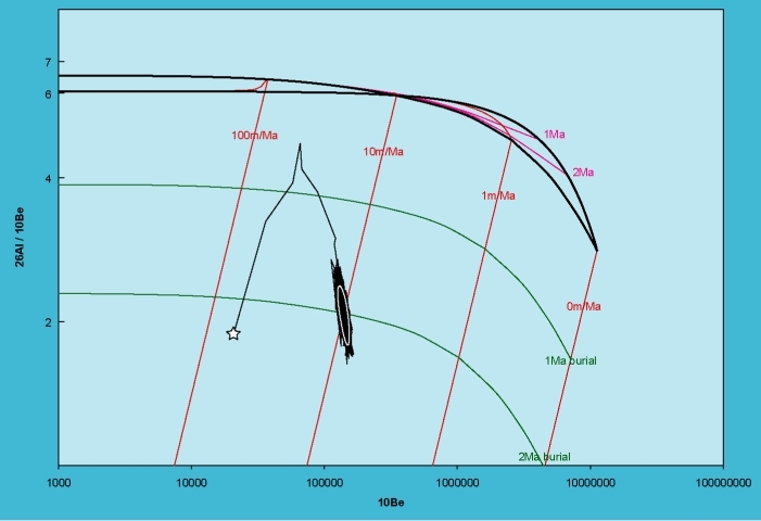
If a rock surface gets buried by sediments or covered by ice, it is
shielded from cosmic rays and the concentration of cosmogenic
radionuclides decays with time. Such samples plot outside the
steady-state erosion island of the banana plot, in the so-called field
of ``complex exposure history'', a feature which is considered
undesirable by most studies. Other studies, however, intentionally
target complex exposure histories, using radionuclides to date
pre-exposure and burial (e.g., Bierman et al., 1999; Fabel et al.,
2002; Partridge et al., 2003). CosmoCalc calculates burial ages,
either by assuming negligible erosion or steady state erosion
(![]() = 0 or t =
= 0 or t = ![]() , respectively). It does not handle
post-depositional nuclide production.
, respectively). It does not handle
post-depositional nuclide production.
Burial - Exposure dating
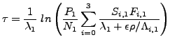
If ![]() = 0, Equation 8 reduces to:
= 0, Equation 8 reduces to:
The easiest case of two-nuclide dating is that of simultaneously
calculating exposure age (t) and burial age (![]() ) with one
radionuclide and one stable nuclide. Because the stable nuclide is
not affected by burial, it can be used to calculate the pre-exposure
age, using Equation 12. This age can then be used to
calculate the burial age:
) with one
radionuclide and one stable nuclide. Because the stable nuclide is
not affected by burial, it can be used to calculate the pre-exposure
age, using Equation 12. This age can then be used to
calculate the burial age:
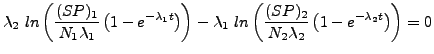
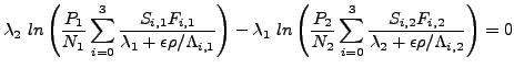
In the case of two radionuclides, CosmoCalc finds t by iteratively solving the following equation using Newton's method:
With
![]() . The solution is then plugged into
Equation 17, using nuclide 1.
. The solution is then plugged into
Equation 17, using nuclide 1.
Burial - Erosion dating
Setting t = ![]() in Equation 8 yields the following
system of non-linear equations for TCN concentrations
in Equation 8 yields the following
system of non-linear equations for TCN concentrations ![]() and
and ![]() :
:
These equations are easy to solve since the variables ![]() and
and
![]() are separated. If nuclide 1 has the shortest half-life
(largest decay constant
are separated. If nuclide 1 has the shortest half-life
(largest decay constant ![]() ), the burial age is written as a
function of the erosion rate
), the burial age is written as a
function of the erosion rate ![]() :
:
The erosion rate is given implicitly by:
CosmoCalc solves Equation 21 for ![]() using
Newton's method and then plugs this value into Equation 20.
If
using
Newton's method and then plugs this value into Equation 20.
If
![]() , then
, then ![]() is used instead of
is used instead of ![]() in
Equation 20.
in
Equation 20.
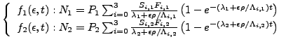
Assuming zero burial (![]() = 0) yields the following system of
equations
= 0) yields the following system of
equations ![]() and
and ![]() :
:
It is impossible to solve these equations for exposure age (t) and
erosion rate (![]() ) separately. Instead, CosmoCalc implements
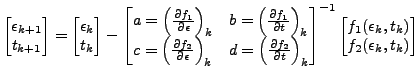
the two-dimensional version of the Newton-Raphson algorithm:
) separately. Instead, CosmoCalc implements
the two-dimensional version of the Newton-Raphson algorithm:
With
 the Jacobian matrix, which
is also used for error propagation.
the Jacobian matrix, which
is also used for error propagation.
Error propagation is less straightforward in the two-dimensional case
than in the single nuclide case (Section 5). The
bijection from (![]() ,
,![]() )-space to (
)-space to (![]() ,t)-space is not
orthogonal, particularly in the case of age-erosion dating (Section
5). For this reason, it is only possible to
analytically compute upper bounds for
,t)-space is not
orthogonal, particularly in the case of age-erosion dating (Section
5). For this reason, it is only possible to
analytically compute upper bounds for
![]() ,
,
![]() and
and ![]() (t):
(t):
with x and y placeholders for ![]() and t or
and t or ![]() ,
respectively, and
,
respectively, and
![]() the absolute values of the
matrix
the absolute values of the
matrix
![]() . In the case of age-erosion dating,
the confidence intervals for t and
. In the case of age-erosion dating,
the confidence intervals for t and ![]() are very wide, often too
wide to be useful. Therefore, it can be more productive to solve each
quantity separately instead of simultaneously. Thus, using equations
11 and 13, it is possible to estimate minimum
exposure ages and maximum erosion rates (e.g., Nishiizumi et al.,
1991). However, for burial dating there is no choice and we must
simultaneously solve for
are very wide, often too
wide to be useful. Therefore, it can be more productive to solve each
quantity separately instead of simultaneously. Thus, using equations
11 and 13, it is possible to estimate minimum
exposure ages and maximum erosion rates (e.g., Nishiizumi et al.,
1991). However, for burial dating there is no choice and we must
simultaneously solve for ![]() and
and ![]() or t.
or t.
In addition to Newton's method, CosmoCalc offers a second way of
solving equations 19 and 22
by means of Monte Carlo simulation, implementing the
Metropolis-Hastings algorithm (Metropolis et al., 1953; Tarantola,
2004). The Metropolis-Hastings algorithm is a so-called Bayesian MCMC
(Markov Chain Monte Carlo) method. It not only finds the best solution
to the system of non-linear equations, but actually explores the
entire solution space. If the ``Metropolis'' option of the
Age-Erosion function is selected, CosmoCalc generates 1000
``acceptable'' solutions to Equation 19 or
22, where ``acceptable'' is defined by the
bivariate normal likelihood of the forward-modeled TCN concentrations
(Figure 3). The last 900 of these solutions
are then ranked according to their likelihood. For a 95% confidence
interval, those solutions with the lowest 5% likelihoods of the 900
results are discarded, leaving 855 values for ![]() , t or
, t or ![]() .
The minimum and maximum values of these 855 numbers are the lower and
upper bounds, respectively, of the simultaneous 95% confidence
intervals. In contrast with the symmetric confidence intervals given
by equation 24, the MCMC confidence limits are always
greater than or equal to zero. However, as said before, the 95%
confidence intervals can be very wide especially in the case of
age-erosion dating.
.
The minimum and maximum values of these 855 numbers are the lower and
upper bounds, respectively, of the simultaneous 95% confidence
intervals. In contrast with the symmetric confidence intervals given
by equation 24, the MCMC confidence limits are always
greater than or equal to zero. However, as said before, the 95%
confidence intervals can be very wide especially in the case of
age-erosion dating.
|
An a posteriori modification of the banana plots
Section 4 discussed the construction of
![]() Al-
Al-![]() Be and
Be and ![]() Ne-
Ne-![]() Be banana plots. To plot
samples from different field locations (with different latitude,
elevation and shielding conditions) together on the same banana plot,
it is necessary to scale the TCN concentrations to SLHL. In other
words, each TCN concentration must be divided by an appropriate
scaling factor, the so-called ``effective scaling factor''
Be banana plots. To plot
samples from different field locations (with different latitude,
elevation and shielding conditions) together on the same banana plot,
it is necessary to scale the TCN concentrations to SLHL. In other
words, each TCN concentration must be divided by an appropriate
scaling factor, the so-called ``effective scaling factor'' ![]() (Equation 5):
(Equation 5):
With ![]() the measured TCN concentration, and
the measured TCN concentration, and ![]() the
equivalent TCN concentration which would be measured had the sample
been collected from SLHL. In the case of zero erosion,
the
equivalent TCN concentration which would be measured had the sample
been collected from SLHL. In the case of zero erosion, ![]() =
=
![]() / (
/ (
![]() ).
This is no longer true when
).
This is no longer true when
![]() , because the relative
contributions of neutron spallation, slow and fast muons change below
the surface. This is the ``fractionation'' effect that was discussed
in Section 4 and quantified by Equation
10. For example, consider the case of two high
latitude, high elevation samples, one with negligible erosion
(
, because the relative
contributions of neutron spallation, slow and fast muons change below
the surface. This is the ``fractionation'' effect that was discussed
in Section 4 and quantified by Equation
10. For example, consider the case of two high
latitude, high elevation samples, one with negligible erosion
(![]() =0) and one with non-zero erosion (
=0) and one with non-zero erosion (
![]() ).
Because the relative importance of neutron spallation increases with
decreasing erosion rate, and neutrons are more important (relative to
muons) at higher elevations,
).
Because the relative importance of neutron spallation increases with
decreasing erosion rate, and neutrons are more important (relative to
muons) at higher elevations, ![]() will be greater for the
zero-erosion than for the non-zero erosion case. CosmoCalc first
solves Equation 19 or 22 for
will be greater for the
zero-erosion than for the non-zero erosion case. CosmoCalc first
solves Equation 19 or 22 for
![]() and
and ![]() or t, whichever fits the measured TCN
concentrations best. Plugging these solutions into Equation
4 yields the equivalent TCN concentration at SLHL.
or t, whichever fits the measured TCN
concentrations best. Plugging these solutions into Equation
4 yields the equivalent TCN concentration at SLHL.
![]() is then given by Equation 25.
is then given by Equation 25.