Shielding corrections

The scaling factors discussed in the previous section allow the calculation of TCN production rates at any location on the Earth's surface, assuming that the sample is a slab of zero thickness taken from a horizontal planar surface. If these assumption are not fulfilled, the SLHL production rates must be multiplied by a second set of correction factors, quantifying the extent to which the cosmic rays were blocked. CosmoCalc implements three such correction factors: topographic shielding, self shielding and snow cover.

Topographic shielding

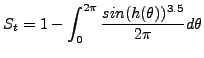
Two kinds of topographic shielding corrections can be distinguished for (a) samples taken from a tilted rather than horizontal surface, and (b) samples that are located in the vicinity of topographic irregularities. CosmoCalc follows the approach of Balco and Stone (2007) (their Matlab function skyline.m) and treats these two effects together using the following equation:

$$S_t = 1 - \int_0^{2 \pi}\frac{sin(h(\theta))^{3.5}}{2 \pi}d\theta$$ (1)

With h($\theta$) the ``horizon'' in the azimuthal direction $\theta$, i.e. either the elevation (in radians) of the topography or the sloping sample surface, whichever is greatest. Sometimes, an exponent of 2.3 is used instead of 3.5 in Equation 1 (Staudacher and Allègre, 1993). CosmoCalc treats this exponent as a variable, which can be changed in the Settings form (Section 7). In practice, the integral of Equation 1 is solved by linear interpolation between a finite number of azimuth/elevation measurements. The input needed by CosmoCalc is two mandatory columns of strike and dip (in degrees, where the strike is 90 degrees less than the direction of the dip), followed by an optional series of topographic azimuth/elevation measurements (in degrees). There is no restriction on the total number of measurements, provided they come in multiples of two.

Self-shielding

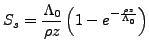
Cosmic rays are rapidly attenuated as they travel through matter, causing TCN production rates to vary greatly with depth below the rock/air contact. They must be integrated over the actual sample thickness and scaled to the surface production rates before an exposure age can be calculated. Different reaction mechanisms are associated with different attenuation lengths. Gosse and Philips (2001) consider four kinds of thickness corrections, for spallogenic, thermal and epithermal neutrons, and muons. Because self-shielding corrections are generally small, CosmoCalc considers only the spallogenic neutron reactions:

$$S_s = \frac{\Lambda_0}{\rho z} \left(1 - e^{-\frac{\rho z}{\Lambda_0}}\right)$$ (2)

with $\Lambda_0$ the spallogenic neutron attenuation length (default value 160 g/cm$^2$), $\rho$ the rock density (default value 2.65 g/cm$^3$) and z the sample thickness (in cm). Neglecting the remaining pathways makes little difference, with the possible exception of $^{36}$Cl, because the latter can be strongly affected by thermal neutron fluxes, which are currently ignored by CosmoCalc.

Snow cover

Perhaps the most popular and powerful application of TCN techniques is the dating of glacial moraines (e.g., Gosse et al., 1995; Schäfer et al., 1999). These features are generally located at high latitudes or elevations, where snow cover poses a potential problem. The snow correction is similar to the self-shielding correction with the important difference that the former is highly variable with time. 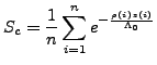Given n (e.g., 12 for monthly or 4 for seasonal) measurements of average snow thickness z and density $\rho$, CosmoCalc computes the snow correction factor $S_c$ as follows:

$$S_c = \frac{1}{n} \sum_{i=1}^{n} e^{-\frac{\rho(i) z(i)}{\Lambda_0}}$$ (3)