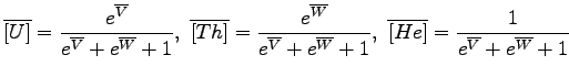
The age-equations 2, 3 and
5 do not specify the measurement units of [U], [Th]
and [He]. These can be expressed in moles or moles/g, but they can
also be non-dimensionalized by normalization to a constant sum: [U']
![]() [U]/([U]+[Th]+[He]), [Th']
[U]/([U]+[Th]+[He]), [Th'] ![]() [Th]/([U]+[Th]+[He]) and
[He']
[Th]/([U]+[Th]+[He]) and
[He'] ![]() [He]/([U]+[Th]+[He]) so that [U'] + [Th'] + [He'] = 1.
Therefore, U, Th and He form a ternary system, can be plotted on a
ternary diagram, and are subject to the peculiar mathematics of the
ternary dataspace. In a three-component system (A+B+C=1), increasing
one component (e.g., A) causes a decrease in the two other components
(B and C). Another consequence of so-called data closure is
that the arithmetic mean of compositional data has no physical meaning
(Weltje, 2002).
[He]/([U]+[Th]+[He]) so that [U'] + [Th'] + [He'] = 1.
Therefore, U, Th and He form a ternary system, can be plotted on a
ternary diagram, and are subject to the peculiar mathematics of the
ternary dataspace. In a three-component system (A+B+C=1), increasing
one component (e.g., A) causes a decrease in the two other components
(B and C). Another consequence of so-called data closure is
that the arithmetic mean of compositional data has no physical meaning
(Weltje, 2002).
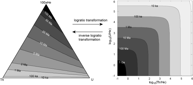
Plotting the (U-Th)/He age equation on ternary diagrams
Following the nomenclature of Aitchison (1986), the ternary diagram is
a 2-simplex (![]() ) (also see Weltje, 2002). The very fact
that it is possible to plot ternary data on a two-dimensional sheet of
paper tells us that the sample space really has only two, and not
three dimensions. As a solution to the compositional data problem,
Aitchison (1986) suggested to transform the data from
) (also see Weltje, 2002). The very fact
that it is possible to plot ternary data on a two-dimensional sheet of
paper tells us that the sample space really has only two, and not
three dimensions. As a solution to the compositional data problem,
Aitchison (1986) suggested to transform the data from ![]() to
to
![]() using the logratio transformation. After
performing the desired (``traditional'') statistical analysis on the
transformed data in
using the logratio transformation. After
performing the desired (``traditional'') statistical analysis on the
transformed data in
![]() , the results can be transformed
back to
, the results can be transformed
back to ![]() using the inverse logratio transformation (Figure
3). Implementation details about the logratio
transformation will be given in Section 4.
using the inverse logratio transformation (Figure
3). Implementation details about the logratio
transformation will be given in Section 4.
Ternary diagrams and logratio plots are useful tools for visualizing
U-Th-He data and the (U-Th)/He age equation. Thus, it can be shown
that the linear age-equation is accurate to better than 1% for ages
up to 100 Ma (Figure 4.a) whereas the equation of
Meesters and Dunai (2005) reaches the same accuracy at 1 Ga (Figure
4.b). Figure 4.c represents a warning
against applying the ![]() -ejection correction after, rather than
before the age-calculation. This causes a partial ``linearization''
of the age-equation and results in a loss of accuracy. For example,
dividing an uncorrected (U-Th)/He age by an
-ejection correction after, rather than
before the age-calculation. This causes a partial ``linearization''
of the age-equation and results in a loss of accuracy. For example,
dividing an uncorrected (U-Th)/He age by an ![]() -retention factor
F
-retention factor
F![]() of 0.7 results in a misfit that is 30% of the linear age
equation misfit. To take full advantage of the accuracy of the exact
age equation, one must divide [He] by F
of 0.7 results in a misfit that is 30% of the linear age
equation misfit. To take full advantage of the accuracy of the exact
age equation, one must divide [He] by F![]() before calculating
the (U-Th)/He age.
before calculating
the (U-Th)/He age.
|
|
(a) 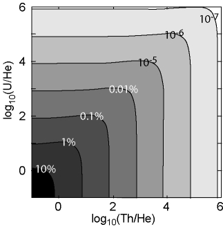 (b)
(b) 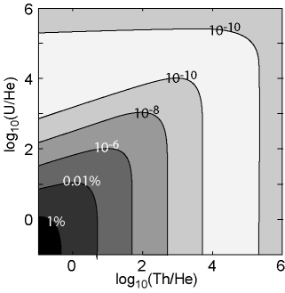 (c)
(c) 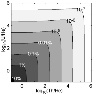
|
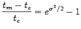
The central age
The logratio transformation is useful for more than just the purpose
of visualization. It provides a fourth and arguably best way to
calculate the average age of a population of single-grain (U-Th)/He
measurements. The central age is calculated from the
``average'' U-Th-He composition of the dataset, where ``average'' is
defined as the geometric mean of the single grain U, Th and He
measurements. The geometric mean of compositional data equals the
arithmetic mean of logratio transformed data.
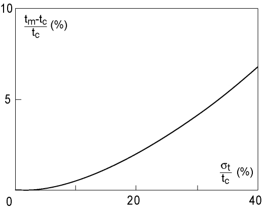
How important is the difference between the arithmetic mean age and
the central age? To simplify this question, consider the special case
of a sample with only one radioactive parent, say Th. Assume that W =
ln([He]/[Th]) is normally distributed with mean ![]() and standard
deviation
and standard
deviation ![]() . Using the linearized age equation for clarity,
the central age t
. Using the linearized age equation for clarity,
the central age t![]() is given by:
is given by:
with C = 1/(6
![]() ) for Th. Using the first raw moment of
the lognormal distribution (Aitchison and Brown, 1957), the arithmetic
mean age t
) for Th. Using the first raw moment of
the lognormal distribution (Aitchison and Brown, 1957), the arithmetic
mean age t![]() is:
is:
so that the relative difference between t![]() and t
and t![]() is:
is:
Using the second central moment of the lognormal distribution (Aitchison and Brown, 1957), the variance of the single-grain ages is given by:
Plotting
![]() versus
versus ![]() /t
/t![]() reveals that the
central age is systematically younger than the mean age. Fortunately,
the difference is small. For example, for a typical external
reproducibility of
reveals that the
central age is systematically younger than the mean age. Fortunately,
the difference is small. For example, for a typical external
reproducibility of ![]() 25% (e.g.
25% (e.g.
![]() = 11% for
Stock et al., 2006), the expected difference is
= 11% for
Stock et al., 2006), the expected difference is ![]() 1% (Figure
5). Finally, it is interesting to note that the
geometric mean of the log-normal distribution equals its median.
Therefore, the central age asymptotically converges to the median age.
However, typical numbers of replicate analyses are not sufficient for
this approach to be truely beneficial.
1% (Figure
5). Finally, it is interesting to note that the
geometric mean of the log-normal distribution equals its median.
Therefore, the central age asymptotically converges to the median age.
However, typical numbers of replicate analyses are not sufficient for
this approach to be truely beneficial.
|
Application to HF-treated Naxos apatites
We now return to the sample of HF-treated inclusion-bearing apatites
from Naxos that was previously used to illustrate the pooled and
isochron age (Figures 1 and 2). The
raw data and the different steps of the central age calculation are
given in Table 1. We will now walk through the
different parts (labeled a, b and c) of this table.
(a) The upper left part of Table 1 lists the U, Th and
He abundances of 11 single-grain analyses. Their respective
single-grain ages (t) were calculated using the exact age equation,
although the linear age approximation (Equation 3) is
accurate to better than 0.1% for such young ages (Figure
4.a). The pooled U, Th and He abundances are obtained
by simple summation of the constituent grains. Note that the helium
abundances are corrected for ![]() -ejection prior to being
pooled. A nominal
-ejection prior to being
pooled. A nominal ![]() =15% statistical uncertainty is associated
with F
=15% statistical uncertainty is associated
with F![]() , assuming randomly distributed mineral inclusions
(Vermeesch et al., 2007). The pooled abundances were normalized to
unity to facilitate comparison with the geometric mean composition
(see below).
, assuming randomly distributed mineral inclusions
(Vermeesch et al., 2007). The pooled abundances were normalized to
unity to facilitate comparison with the geometric mean composition
(see below).
(b) To calculate the isochron age, the abundances are first rescaled
to units of concentration (e.g. in nmol/g). This removes the bias
towards large grains, which can dominate the pooled age calculation.
The ![]() -production rate P is given by Equation 4. The
linear regression (Figure 2) was done using Isochron
3.0 (Ludwig, 2003), yielding a slope of 12.0
-production rate P is given by Equation 4. The
linear regression (Figure 2) was done using Isochron
3.0 (Ludwig, 2003), yielding a slope of 12.0 ![]() 4.2 Ma with an
intercept of -0.05
4.2 Ma with an
intercept of -0.05 ![]() 0.45 nmol/g He.
0.45 nmol/g He.
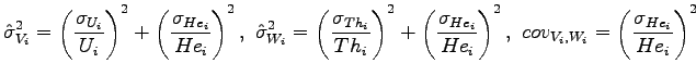
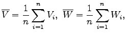
(c) Central ages are somewhat more complicated to calculate than arithmetic mean ages, pooled ages or isochron ages. Therefore, these calculations will be discussed in more detail. First, transform each of the n single grain analyses to logratio space:
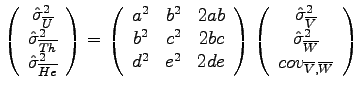
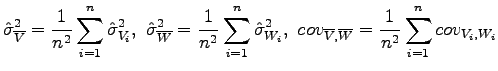
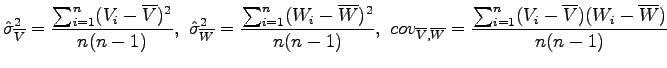
For i = 1,...,n. Note that this transformation can be done irrespective of whether the U, Th and He measurements are expressed in abundance units or in units of concentration. Following standard error propagation, the (co)variances of these quantities are estimated by:
Next, calculate the arithmetic mean of the logratio transformed data:
With the following (co)variances:
Note that equation 14 only propagates the internal (i.e. analytical) uncertainty, and not the external error. Single grain (U-Th)/He ages tend to suffer from overdispersion with respect to the formal analytical precision for a number of reasons (Fitzgerald et al., 2006; Vermeesch et al., 2007). Therefore, it may be better to use an alternative equation propagating the external error:
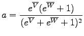
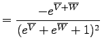
Error-weighting can be done by trivial generalizations of equations 13, 14 and 15, which are implemented in the web-calculator. The geometric mean composition is given by the inverse logratio transformation (Aitchison, 1986; Weltje, 2002):
With variances:
where
 |
 |
||
 |
 |
||
 |
The central age is then simply calculated by plugging
![]() ,
,
![]() and
and
![]() and their
uncertainties into equation 2, 3 or
5.
and their
uncertainties into equation 2, 3 or
5.
As predicted (Figure 5), the arithmetic mean age
is older than the central age. There is less than 2% disagreement
between the arithmetic mean age (![]() 11.58 Ma) and the central age
(
11.58 Ma) and the central age
(![]() 11.38 Ma), and 7% difference between the pooled age (
11.38 Ma), and 7% difference between the pooled age (![]() 11.28 Ma) and the isochron age (
11.28 Ma) and the isochron age (![]() 12.0 Ma).
12.0 Ma).
|
(a) 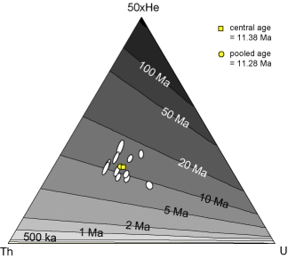 (b)
(b) 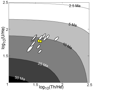
|
![$\displaystyle V_i = ln\left(\frac{[U_i]}{[He_i]}\right),~
W_i = ln\left(\frac{[Th_i]}{[He_i]}\right)$](img48.png)
![$\displaystyle \overline{[U]} = \frac{e^{\overline{V}}}{e^{\overline{V}}+e^{\ove...
...rline{W}}+1},~
\overline{[He]} = \frac{1}{e^{\overline{V}}+e^{\overline{W}}+1}$](img53.png)