For reasons given in the Introduction, ![]() Sm is often neglected
in helium thermochronometry. However, in rare cases it does happen
that apatite contains high abundances of Sm, affecting the helium age
on the percent level. This section will explain how to add a fourth
radioactive parent to the methods described above. The exact age
equation (equation 2) and the present-day helium
production rate (equation 4) can easily be generalized to
include Sm:
Sm is often neglected
in helium thermochronometry. However, in rare cases it does happen
that apatite contains high abundances of Sm, affecting the helium age
on the percent level. This section will explain how to add a fourth
radioactive parent to the methods described above. The exact age
equation (equation 2) and the present-day helium
production rate (equation 4) can easily be generalized to
include Sm:
and
With
![]() the decay constant of
the decay constant of ![]() Sm and all other
parameters as in equations 2 and 4. Using
equation 19, calculating an isochron age for (U-Th-Sm)/He
proceeds in exactly the same way as for the ordinary (U-Th)/He method,
and the same is true for the pooled age. Calculating (U-Th-Sm)/He
central ages is also very similar, although the equations are a bit
longer. In addition to V
Sm and all other
parameters as in equations 2 and 4. Using
equation 19, calculating an isochron age for (U-Th-Sm)/He
proceeds in exactly the same way as for the ordinary (U-Th)/He method,
and the same is true for the pooled age. Calculating (U-Th-Sm)/He
central ages is also very similar, although the equations are a bit
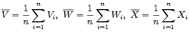
longer. In addition to V![]() and W
and W![]() (equation
11), we define a third logratio variable
X
(equation
11), we define a third logratio variable
X![]() (1
(1![]() i
i![]() n):
n):
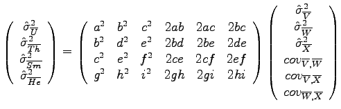
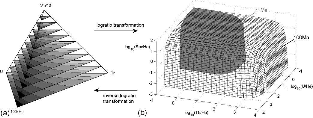
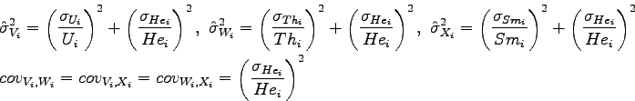
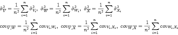
Because there are three instead of two logratio variables, the (U-Th-Sm)/He age equation cannot be visualized on a straightforward bivariate diagram, but forms a set of hypersurfaces in trivariate logratio-space (Figure 7). Likewise, (U-Th-Sm)/He data do not form a ternary, but a tetrahedral system in compositional dataspace (Figure 7). Generalizing the (co)variances of equation 12:
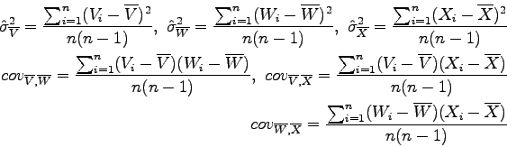
Calculating the arithmetic logratio-means:
The (co-)variances of the logratio-means, propagating only the internal error:
The (co-)variances of the logratio-means, propagating the external error:
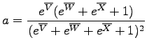
The inverse logratio-transformation:
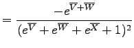
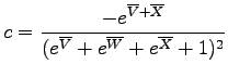
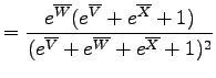
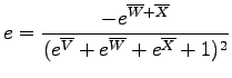
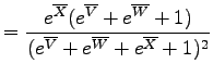
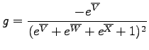
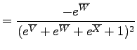
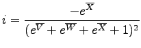
Finally, calculating the standard error propagation of the geometric mean compositions:
with
 |
 |
||
 |
 |
||
 |
 |
||
 |
 |
||
 |
An example of a well-behaved (U-Th-Sm)/He dataset from the Fish Lake
Valley apatite standard (provided by Prof. Daniel Stockli, University
of Kansas) is given in the web-calculator (
http://pvermees.andropov.org/central). The arithmetic mean of 28
single-grain ages is 6.36 ![]() 0.11 Ma, the pooled age 6.43
0.11 Ma, the pooled age 6.43 ![]() 0.21 Ma, the isochron ages 6.44
0.21 Ma, the isochron ages 6.44 ![]() 0.67 Ma (with an intercept of
-0.005
0.67 Ma (with an intercept of
-0.005 ![]() 0.056 fmol/
0.056 fmol/![]() g, and the central age 6.41
g, and the central age 6.41 ![]() 0.14
Ma. Note that the central age is older and not younger than the
arithmetic mean age. This indicates that random variations exceed the
very small systematic difference between the arithmetic and geometric
mean compositions. However, the central age probably still is more
accurate than the arithmetic mean age because it is less sensitive to
outliers.
0.14
Ma. Note that the central age is older and not younger than the
arithmetic mean age. This indicates that random variations exceed the
very small systematic difference between the arithmetic and geometric
mean compositions. However, the central age probably still is more
accurate than the arithmetic mean age because it is less sensitive to
outliers.
|
![\begin{displaymath}\begin{split}[He]= \left( 8\frac{137.88}{138.88}\left(e^{\lam...
...[Th] + 0.1499\left(e^{\lambda_{147}t}-1\right)[Sm]
\end{split}\end{displaymath}](img66.png)
![$\displaystyle P = \left( 8\frac{137.88}{138.88}\lambda_{238} +
\frac{7}{138.88}\lambda_{235} \right) [U]+
6\lambda_{232}[Th] + 0.1499\lambda_{147}[Sm]$](img67.png)
![$\displaystyle V_i = ln\left(\frac{[U_i]}{[He_i]}\right),~
W_i = ln\left(\frac{[Th_i]}{[He_i]}\right),~
X_i = ln\left(\frac{[Sm_i]}{[He_i]}\right)$](img69.png)
![\begin{displaymath}\begin{split}
& \overline{[U]} = \frac{e^{\overline{V}}}{e^{...
...\overline{V}}+e^{\overline{W}}+e^{\overline{X}}+1}
\end{split}\end{displaymath}](img74.png)