In practice, the PDF can never be precisely known, because that would require an exhaustive sampling of the detrital population. Therefore, we must work with estimates of the PDF based on a finite sample of detrital ages (typically tens to hundreds of ages). Besides limited data, measurement uncertainty is a second factor reducing the precision of density estimates. The most popular estimators of probability density are histograms and ``kernel density plots'' [e.g., Silverman, 1986]. Both of these methods apply some degree of ``smoothing'' to the data, either by binning them into a histogram, or by assigning a Gaussian uncertainty distribution to each measurement:
With N(t
![]() ) the normal distribution of t with mean
) the normal distribution of t with mean ![]() and standard deviation
and standard deviation ![]() , and t
, and t![]() and
and ![]() (t
(t![]() )
the measured ages and their respective 1-
)
the measured ages and their respective 1-![]() uncertainties. To
illustrate the different approaches to detrital thermochronological
density estimation, consider the degenerate case of a ``diving board''
hypsometry: all detrital grains are derived from a single elevation,
corresponding to a single ``true'' age t
uncertainties. To
illustrate the different approaches to detrital thermochronological
density estimation, consider the degenerate case of a ``diving board''
hypsometry: all detrital grains are derived from a single elevation,
corresponding to a single ``true'' age t![]() . The PDF of the true
ages is a delta-function (spike at t
. The PDF of the true
ages is a delta-function (spike at t![]() , zero probability
elsewhere). For further simplification, all grains have identical,
Gaussian measurement uncertainties. In the following, t
, zero probability
elsewhere). For further simplification, all grains have identical,
Gaussian measurement uncertainties. In the following, t![]() =
10Ma so all grains are 10Ma old and have Gaussian measurement
uncertainties of 1Ma.
=
10Ma so all grains are 10Ma old and have Gaussian measurement
uncertainties of 1Ma.
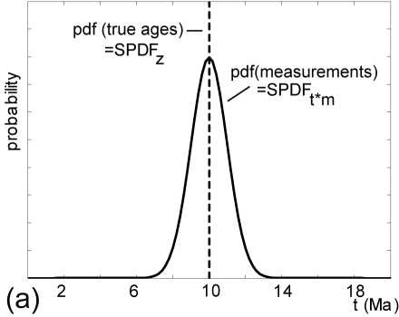
Suppose we have access to an infinite number of measurement from this
detrital population. The PDF of these age measurements can then be
determined by a histogram with infinitessimal binwidth or a kernel
density estimate with infinitessimal ![]() . Note that the PDF of
the measurements is not the same as the PDF of the underlying
ages (Figure 3.a). Unless we deconvolve
the measurement uncertainties, the measurement distribution will
always be a ``smoothed'' version of the ``true'' age distribution. In
our toy example, the age distribution is a delta-function at 10
Ma, whereas the measurement distribution is a Gaussian
distribution with mean 10 Ma and standard deviation 1 Ma (Figure
3.a).
. Note that the PDF of
the measurements is not the same as the PDF of the underlying
ages (Figure 3.a). Unless we deconvolve
the measurement uncertainties, the measurement distribution will
always be a ``smoothed'' version of the ``true'' age distribution. In
our toy example, the age distribution is a delta-function at 10
Ma, whereas the measurement distribution is a Gaussian
distribution with mean 10 Ma and standard deviation 1 Ma (Figure
3.a).
|
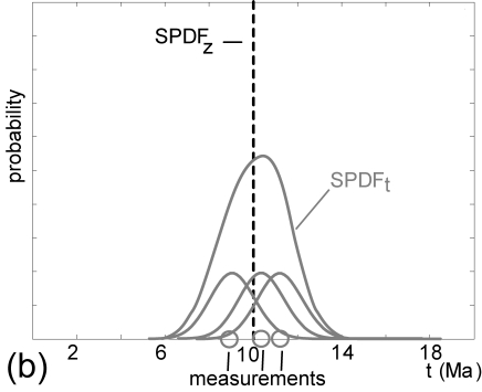
Given a set of age data, the Gaussian kernel density estimator stacks
a bell curve on top of each measurement (Equation 2 and
Figure 3.b). Repeating this for a large number
of measurements drawn from our ``diving board'' hypsometry yields a
Gaussian distribution with mean 10 Ma and standard deviation ![]() =
=
 . Thus,
 ![]() is ``double-smoothed'': once by the measurement uncertainties, and a
second time by the construction of the kernel density estimator. The
amount of additional smoothing depends on the parameter
is ``double-smoothed'': once by the measurement uncertainties, and a
second time by the construction of the kernel density estimator. The
amount of additional smoothing depends on the parameter ![]() .
Although it can be shown that
.
Although it can be shown that ![]() = 0.6 is an optimal value [
Silverman, 1986; Brandon, 1996], previous studies by Brewer et al. [2003], Ruhl and Hodges [2005] and Stock
et al. [2006] have used
= 0.6 is an optimal value [
Silverman, 1986; Brandon, 1996], previous studies by Brewer et al. [2003], Ruhl and Hodges [2005] and Stock
et al. [2006] have used ![]() = 1, and so does Figure
3.b. Ruhl and Hodges [2005] gave this
curve the name ``Synoptic Probability Density Function'' (SPDF).
These authors distinguish between three kinds of SPDF. SPDF
= 1, and so does Figure
3.b. Ruhl and Hodges [2005] gave this
curve the name ``Synoptic Probability Density Function'' (SPDF).
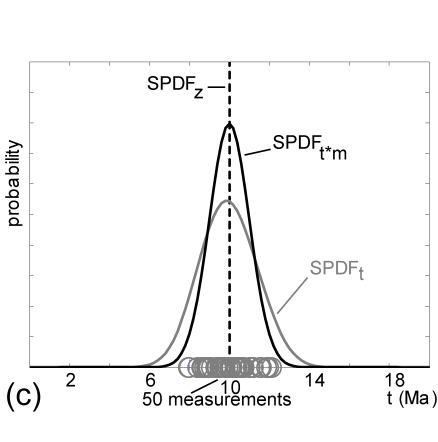
These authors distinguish between three kinds of SPDF. SPDF![]() is
the true underlying age distribution, in the hypothetical case of
errorless measurements (dashed lines in Figure
3). In our toy example, SPDF
is
the true underlying age distribution, in the hypothetical case of
errorless measurements (dashed lines in Figure
3). In our toy example, SPDF![]() is a delta
function. SPDF
is a delta
function. SPDF![]() is the kernel density estimator generated by
Equation 2 (gray lines in Figure
3). Finally, SPDF
is the kernel density estimator generated by
Equation 2 (gray lines in Figure
3). Finally, SPDF![]() effectively is the
PDF of the measurements (black lines in Figure
3). Because SPDF
effectively is the
PDF of the measurements (black lines in Figure
3). Because SPDF![]() is only smoothed
once, whereas SPDF
is only smoothed
once, whereas SPDF![]() is smoothed twice, SPDF
is smoothed twice, SPDF![]() is a biased estimator of SPDF
is a biased estimator of SPDF![]() (Figure
3.c).
(Figure
3.c).
One of the requirements for the application of Gaussian kernel density
estimation is that the measurement uncertainties are normally
distributed. This may be a reasonable assumption for
![]() Ar/
Ar/![]() Ar thermochronology, but not necessarily for fission
tracks, which are governed by a Poisson process. However, by using
the logistic transform, a set of fission track data can be recast in
terms of a new parameter z [Brandon, 1996], which is estimated
by
Ar thermochronology, but not necessarily for fission
tracks, which are governed by a Poisson process. However, by using
the logistic transform, a set of fission track data can be recast in
terms of a new parameter z [Brandon, 1996], which is estimated
by
where ![]() is the decay constant of
is the decay constant of ![]() U
(=1.55125
U
(=1.55125![]() 10
10![]() a
a![]() ),
), ![]() a (zeta) calibration
factor measured on an AFT age standard, g a geometric factor (=0.5),
N
a (zeta) calibration
factor measured on an AFT age standard, g a geometric factor (=0.5),
N![]() the number of spontaneous fission tracks, N
the number of spontaneous fission tracks, N![]() the number of
induced tracks in a mica detector and
the number of
induced tracks in a mica detector and ![]() the induced track
density of a glass standard that was irradiated along with the sample.
N
the induced track
density of a glass standard that was irradiated along with the sample.
N![]() and N
and N![]() are Poisson variables, but
are Poisson variables, but ![]() is normally
distributed with standard error
is normally
distributed with standard error