Although Chayes (1949, 1960, 1971) made significant contributions to
the compositional data problem, the real breakthrough was made by
Aitchison (1982, 1986). Aitchison argues that N-variate data
constrained to a constant sum form an N-1 dimensional sample space or
simplex. An example of a simplex for N=3 is the ternary diagram
(e.g., Weltje, 2002). The very fact that it is possible to plot
ternary data on a two-dimensional sheet of paper tells us that the
sample space really has only two, and not three dimensions. The
``traditional'' statistics of real space (
![]() ) do no longer
work on the simplex (
) do no longer
work on the simplex (
![]() ). Figure
5 shows the breakdown of the calculation
of 100(1-
). Figure
5 shows the breakdown of the calculation
of 100(1-![]() )% confidence intervals on
)% confidence intervals on
![]() . Treating
. Treating
![]() the same way as
the same way as
![]() yields 95% confidence
polygons that partly fall outside the ternary diagram, corresponding
to meaningless negative values of x, y and z.
yields 95% confidence
polygons that partly fall outside the ternary diagram, corresponding
to meaningless negative values of x, y and z.
As a solution to this problem, Aitchison suggested to transform the
data from
![]() to
to
![]() using the
log-ratio transformation (Figure 6). After
performing the desired (``traditional'') statistical analysis on the
transformed data in
using the
log-ratio transformation (Figure 6). After
performing the desired (``traditional'') statistical analysis on the
transformed data in
![]() , the results can then be
transformed back to
, the results can then be
transformed back to
![]() using the inverse log-ratio
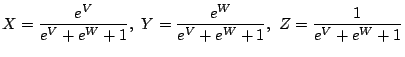
transformation. For example, in the ternary system (X+Y+Z=1), we could
use the transformed values V = log(X/Z) and W = log(Y/Z).
Alternatively, we could also use V=log(X/Y) and W=log(Z/Y), or
V=log(Y/X) and W=log(Z/X). The inverse log-ratio transformation is
given by:
using the inverse log-ratio
transformation. For example, in the ternary system (X+Y+Z=1), we could
use the transformed values V = log(X/Z) and W = log(Y/Z).
Alternatively, we could also use V=log(X/Y) and W=log(Z/Y), or
V=log(Y/X) and W=log(Z/X). The inverse log-ratio transformation is
given by:
The back-transformed confidence regions of Figure
6 are no longer elliptical, but completely
fall within the ternary diagram, as they should. Figure
7 shows an LDA of the synthetic
data of Figures 5 and
6, done the ``wrong'' way (i.e., treating the
simplex as a regular data space). As explained in the previous
section, such an analysis yields linear decision boundaries. 10% of
the training data were misclassified. Figure
8 shows an LDA done the
``correct'' way (i.e., after mapping the data to log-ratio space). The
decision boundaries are still linear, but this time only ![]() 3% of
the training data were misclassified. Because log(Y/Z) and log(X/Z)
are rather hard quantities to interpret, it is a good idea to map the
results back to the ternary diagram using the inverse log-ratio
transformation (Figure 9).
The transformed decision boundaries are no longer linear, but curved.
However, the misclassification rate is still only 3%.
3% of
the training data were misclassified. Because log(Y/Z) and log(X/Z)
are rather hard quantities to interpret, it is a good idea to map the
results back to the ternary diagram using the inverse log-ratio
transformation (Figure 9).
The transformed decision boundaries are no longer linear, but curved.
However, the misclassification rate is still only 3%.
Note that there are two different kinds of constant-sum constraint. The first is a physical one, resulting from the fact that all chemical concentrations add up to 100%. The second is a diagrammatic contraint caused by renormalizing three chosen elements to 100% on a ternary plot. Aitchison's logratio-transform adequately deals with both types of constant sum constraint. The first type is discussed in Sections 5.1 and 5.3, the second in 5.2.