Next: About this document ...
Up: Tectonic discrimination diagrams revisited
Previous: List of Figures
Figure 1:
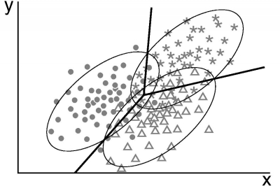
Discriminant analysis of three classes with equal covariance matrices
leads to linear discriminant boundaries. The ellipses mark arbitrary
(e.g., 95%) confidence levels for the underlying populations.
|
|
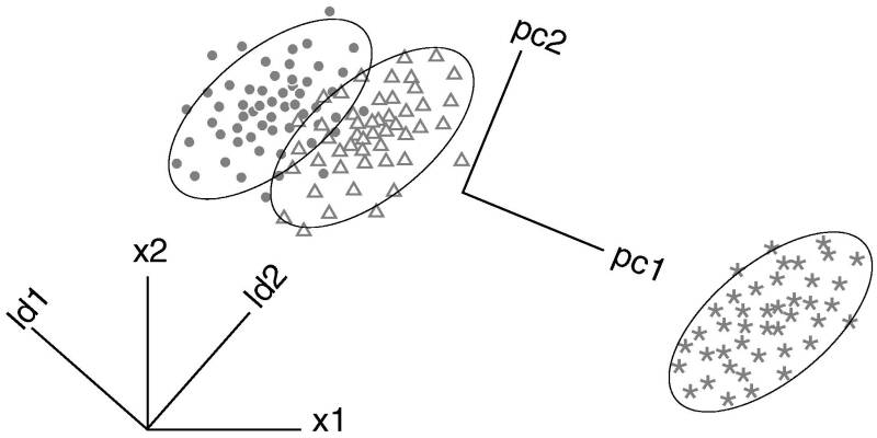
Figure 2:
Similarities and differences between linear discriminant and
principal component analysis. x1 and x2 are the original variables,
pc1 and pc2 are the principal components and ld1 and ld2 are the
linear discriminant functions.
|
|
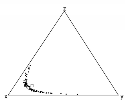
Figure 3:
One of the consequences of the constant-sum constraint of
compositional data is that the arithmetic mean (marked by the open
square) of populations (black dots) has no physical meaning. Instead,
the geometric mean should be used (open circle).
|
|
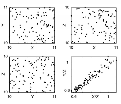
Figure 4:
X, Y and Z are uncorrelated,
uniform random numbers. The strong spurious correlation of the ratios
Y/Z and X/Z is an artifact of the relatively large variance of Z
relative to X, Y and Z.
|
|
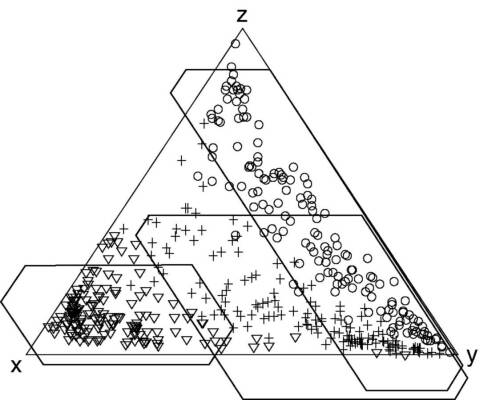
Figure 5:
95% normal confidence regions (e.g., Weltje, 2002) for synthetic
trivariate compositional data partly fall outside the ternary diagram,
a nonsense result illustrating the dangers of performing
``traditional'' statistics on the simplex.
|
|
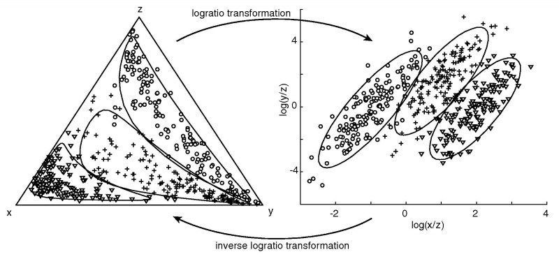
Figure 6:
Following Aitchison (1986), the statistical problems of Figure
5 can be avoided by mapping the data
from the simplex  to
R2 using the logratio
transformation.
to
R2 using the logratio
transformation.
|
|
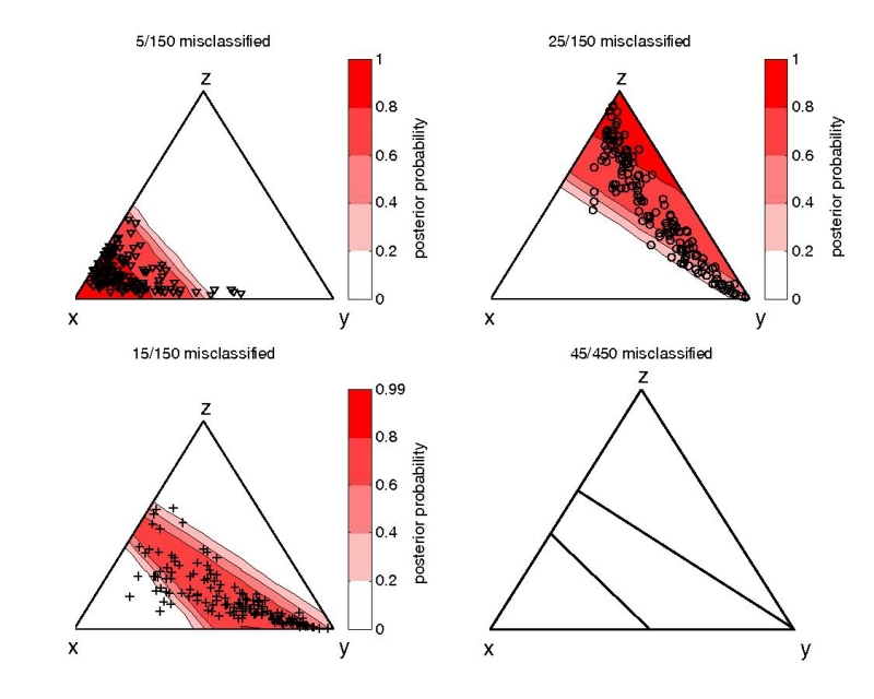
Figure 7:
Linear discriminant analysis using the crude covariance approach
of Figure 5. The red-shaded contours of
the first three ternary diagrams represent the posterior probabilities
for the three classes. The last diagram shows the linear decision
boundaries. 10% of the training data are misclassified.
|
|
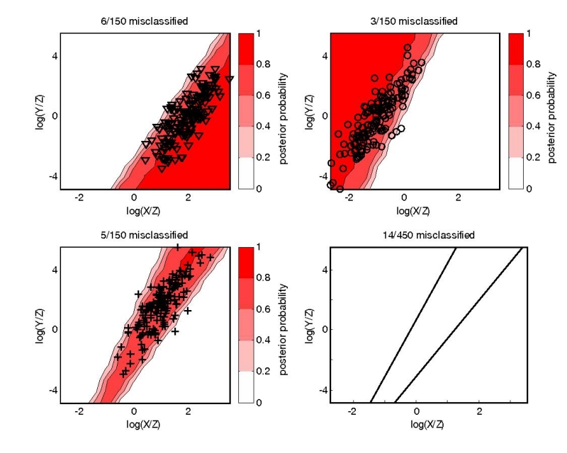
Figure 8:
The same data of Figure 7, mapped
to logratio-space using the approach illustrated by Figure
6. Linear discriminant analysis of these
bivariate data misclassifies only 3% of the training data.
|
|
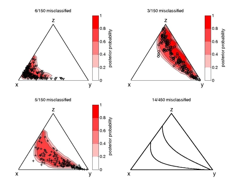
Figure 9:
Mapping the results of Figure 8
back to the ternary diagram with the inverse logratio transformation shown on
Figure 6 yields curved posterior densities and
decision boundaries.
|
|
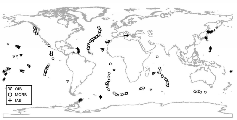
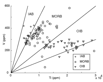
Figure 10:
Locations of the training data: 756 Island Arc (IAB), Mid Ocean Ridge
(MORB) and Ocean Island (OIB) Basalts.
|
|
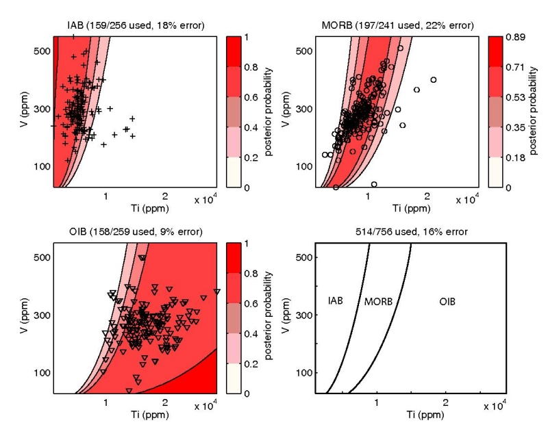
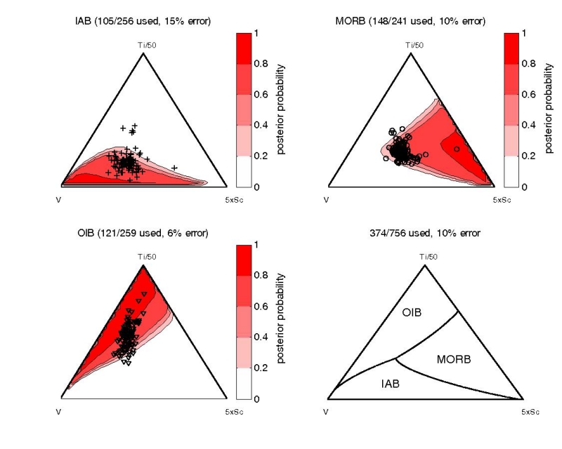
Figure 11:
Linear discriminant analysis (LDA) of the Ti-V system of Shervais
(1982). The red-shaded contours on the first three subplots show the
posterior probability of a particular ``class'' (IAB, MORB, or OIB)
given the training set of 756 basalt samples and a uniform prior. The
last subplot (lower-right) shows the new decision boundaries. The
number of training data used and a resubstitution error estimate are
given for each of the tectonic affinities. The overall resubstitution
error is shown above the lower-right subplot.
|
|
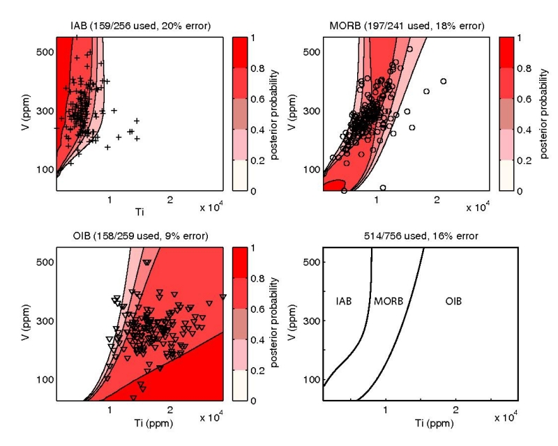
Figure 12:
Quadratic discriminant analysis (QDA) of the Ti-V system. In contrast
with the LDA of Figure 11, each tectonic ``class'' was
allowed to have a different covariance matrix, resulting in slightly
different decision boundaries.
|
|
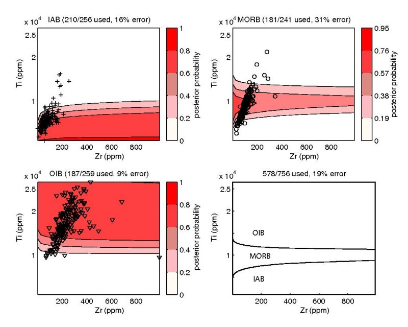
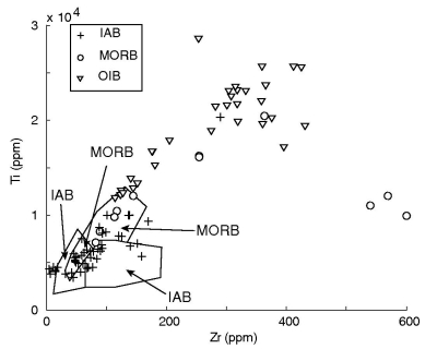
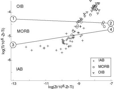
Figure 13:
Linear discriminant analysis of the Ti-Zr system of Pearce and Cann (1973).
|
|
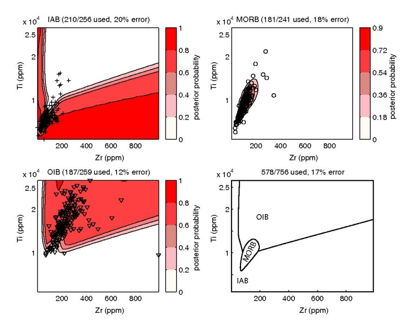
Figure 14:
Quadratic discriminant analysis of the Ti-Zr system.
|
|
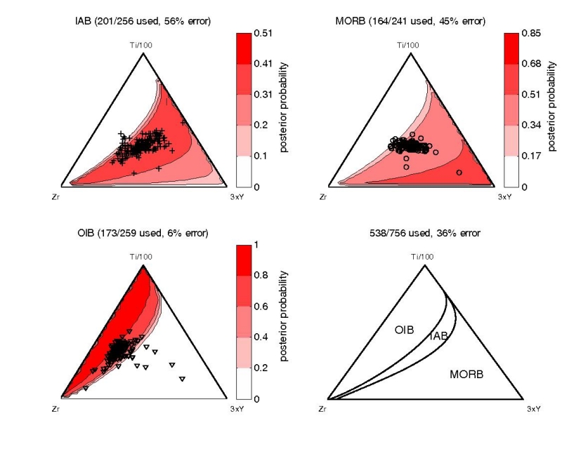
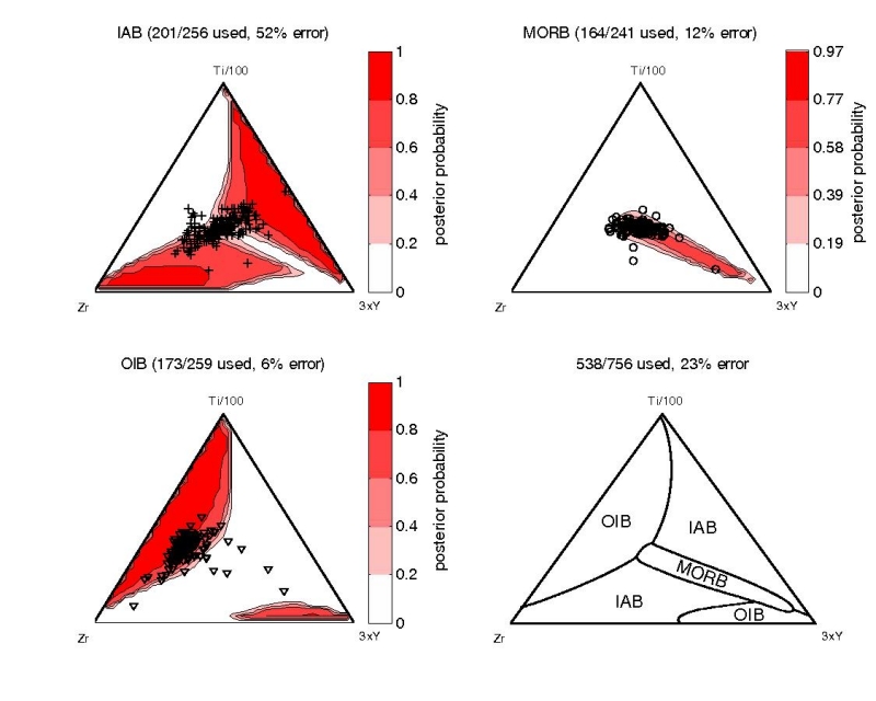
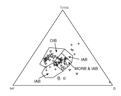
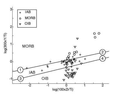
Figure 15:
Linear discriminant analysis of the Ti-Zr-Y system of Pearce and Cann
(1973). The posterior probabilities of nearly all the IAB and MORB
training data are low ( 0.4), resulting in large misclassification
rates for these affinities. As noted by Pearce and Cann (1973), the
Ti-Zr-Y diagram can be used to separate OIBs from IAB/MORBs, but
cannot be used to distinguish between IAB and MORB. For this purpose,
the Ti-Zr diagram (Figure 13) can be used.
0.4), resulting in large misclassification
rates for these affinities. As noted by Pearce and Cann (1973), the
Ti-Zr-Y diagram can be used to separate OIBs from IAB/MORBs, but
cannot be used to distinguish between IAB and MORB. For this purpose,
the Ti-Zr diagram (Figure 13) can be used.
|
|
Figure 16:
Quadratic discriminant analysis of the Ti-Zr-Y system. The OIB/IAB
decision boundary (at low Y) is nearly identical to that of Figure
15, whereas there is a lot more (unstable)
structure at higher Y concentrations.
|
|
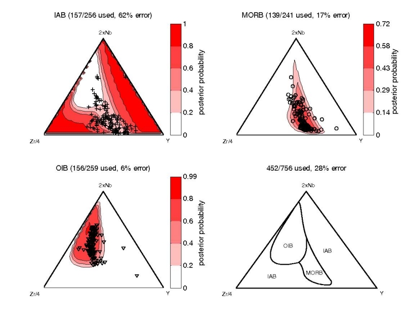
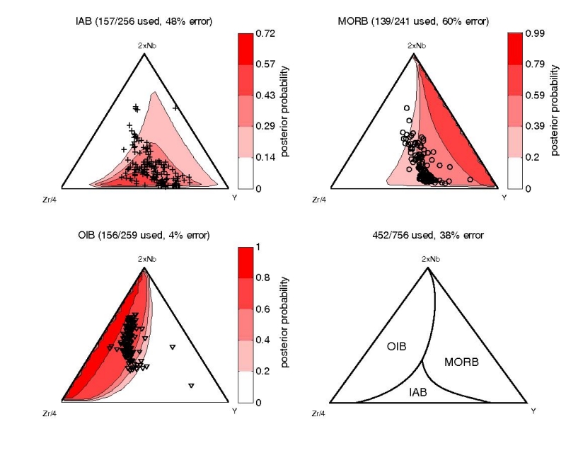
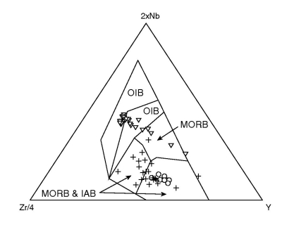
Figure 17:
Linear discriminant analysis of the Zr-Y-Nb system of Meschede
(1986). Like in Figure 15, posterior IAB and MORB
probabilities are low, resulting in high misclassification rates.
|
|
Figure 18:
Quadratic discriminant analysis of the Zr-Y-Nb system.
|
|
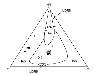
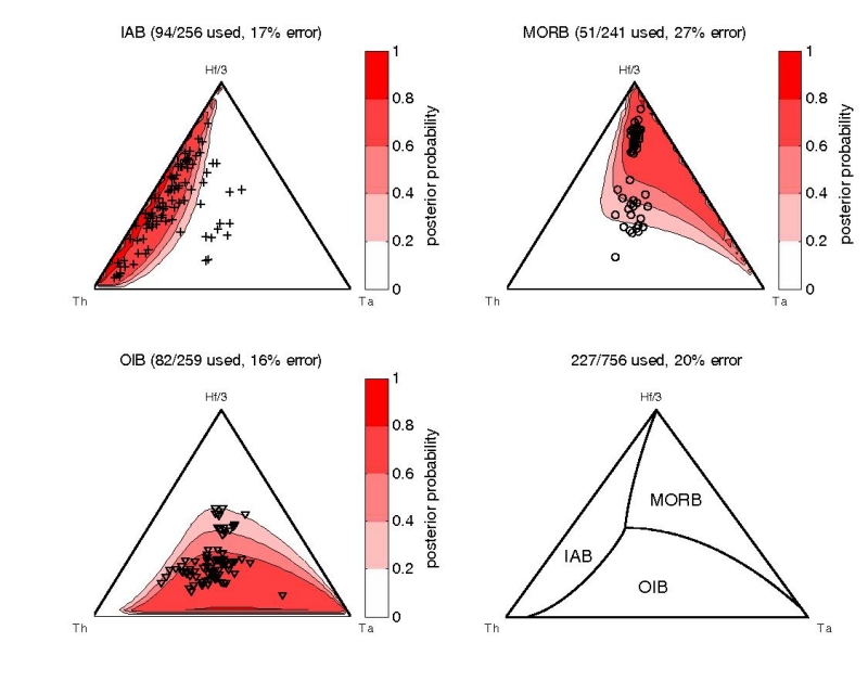
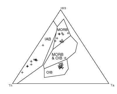
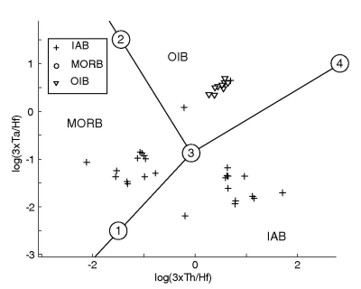
Figure 19:
Linear discriminant analysis of the Th-Ta-Hf system of Wood (1980).
|
|
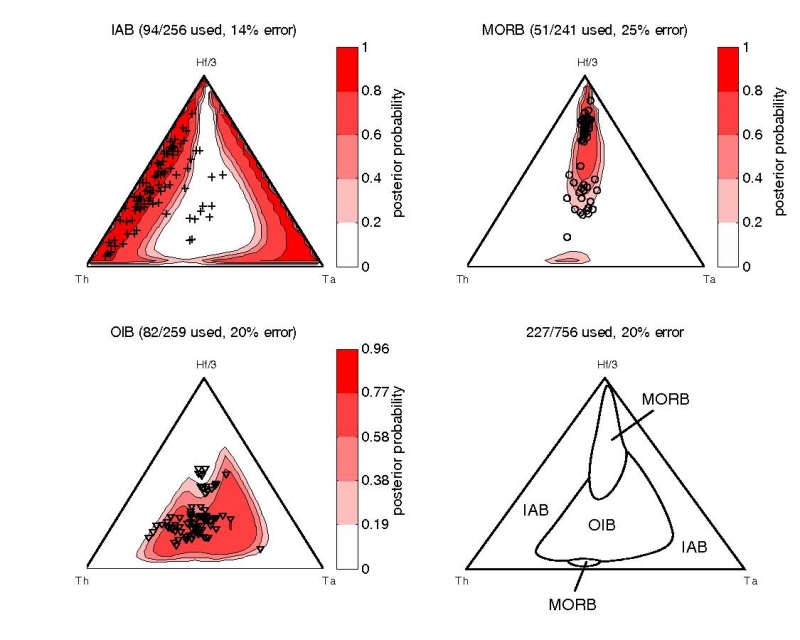
Figure 20:
Quadratic discriminant analysis of the Th-Ta-Hf system.
|
|
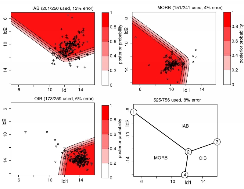
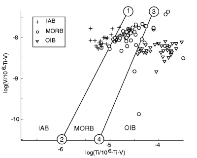
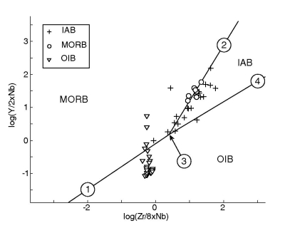
Figure 21:
Linear discriminant analysis of the Ti-Zr-Y-Sr system. ld1 and ld2 are
the two linear discriminant functions, given by Equation
7. They represent two projection planes that optimally
separate the three tectonic affinities (IAB, MORB, and OIB) (see also
Figure 2). The encircled numbers on the lower right
subplot are ``anchor points'' that can be used by the user to
reconstruct the decision boundaries in logratio-space. The ld1/ld2
coordinates of these anchor points are given in Table
6.
|
|
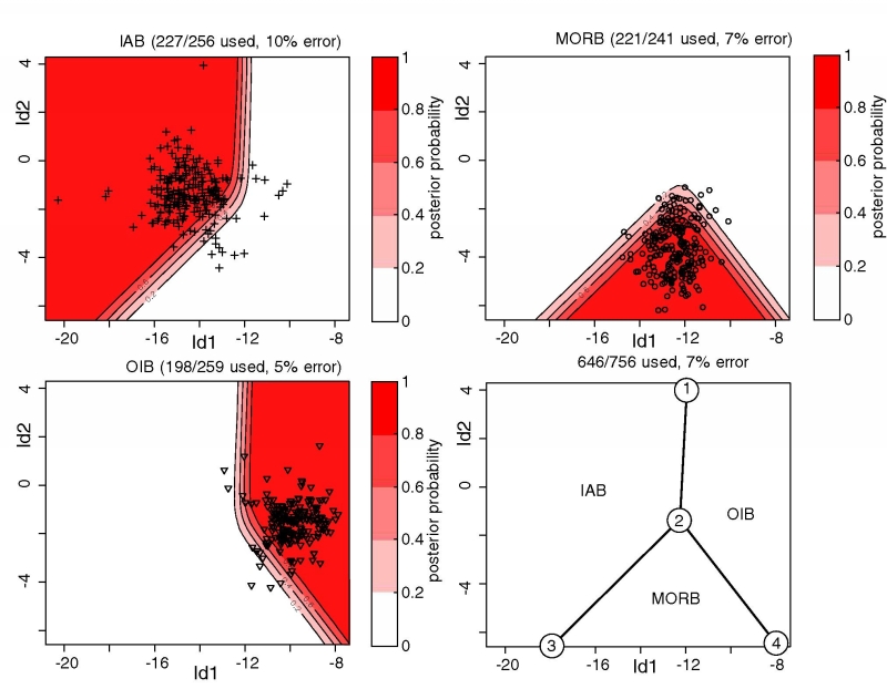
Figure 22:
Linear discriminant analysis of major element data (SiO ,
AlO
,
AlO , TiO, CaO, MgO, MnO, KO, NaO), mapped to
R2 using the logratio transformation. ld1 and ld2 are
given by Equation 8. Anchor points are given in Table
6.
, TiO, CaO, MgO, MnO, KO, NaO), mapped to
R2 using the logratio transformation. ld1 and ld2 are
given by Equation 8. Anchor points are given in Table
6.
|
|
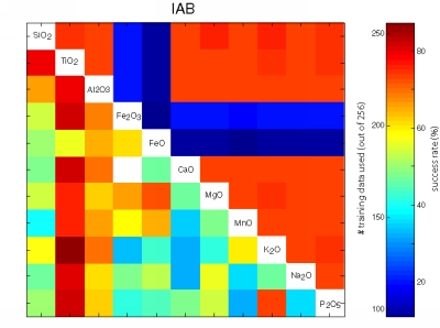
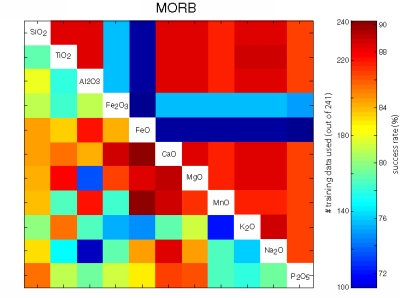
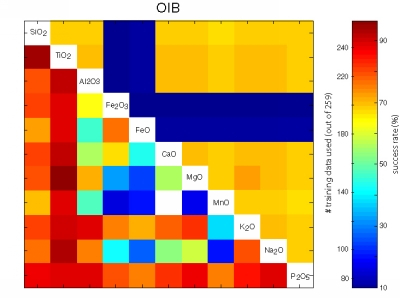
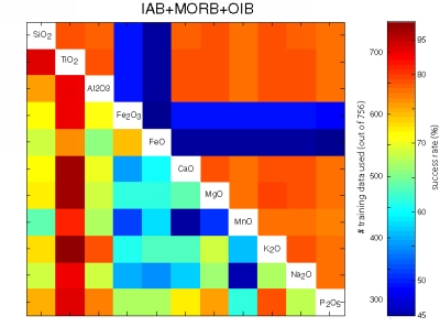
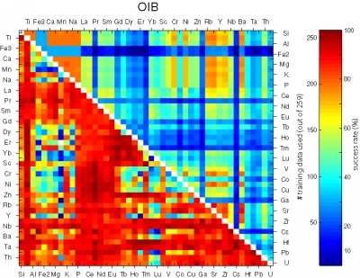
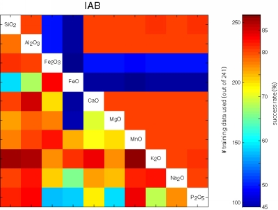
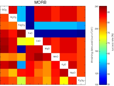
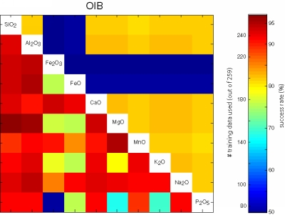
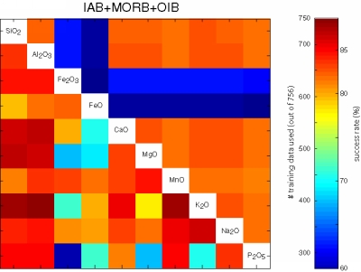
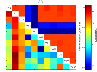
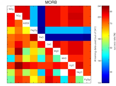
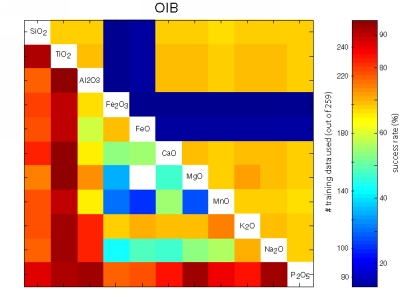
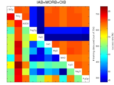
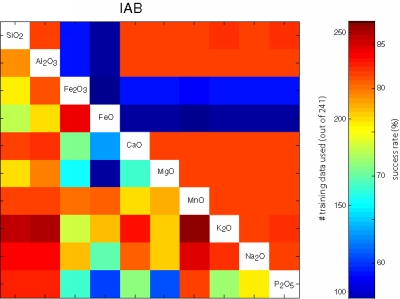
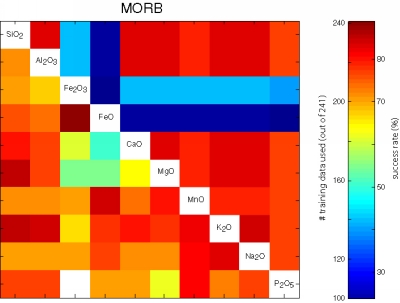
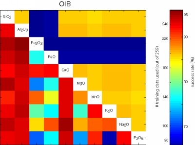
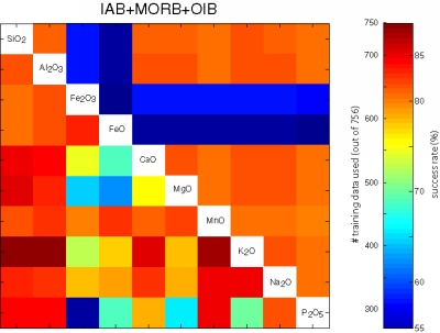
Figure 23:
Visual representation of the performance of all possible bivariate
linear discriminant analyses using the major element data of the
training set of 756 oceanic basalts. The upper right triangular
section of each matrix shows the number of samples that contained both
variables. The lower left sections color-code the fraction of
successfully classified training data.
|
|
Figure 24:
Same as Figure 23,
but for quadratic discriminant analysis.
|
|
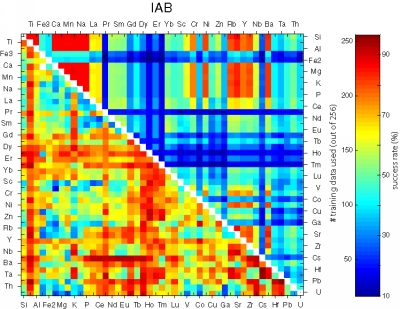
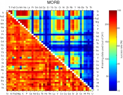
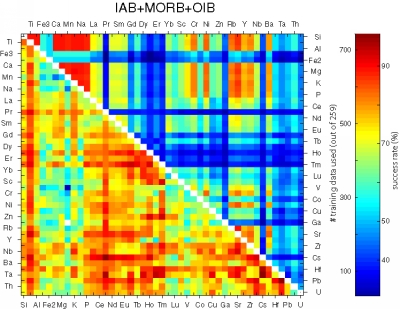
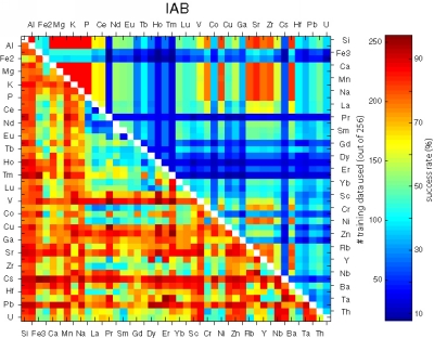
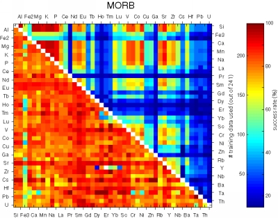
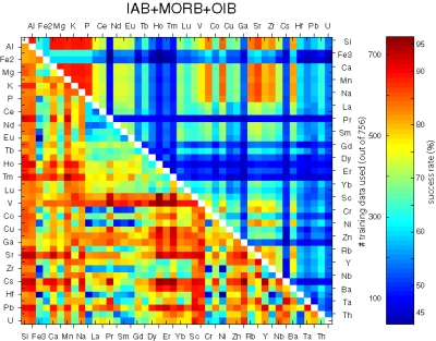
Figure 25:
Matrices showing the performance of all possible bivariate linear
discriminant analyses using combinations of 45 elements.
|
|
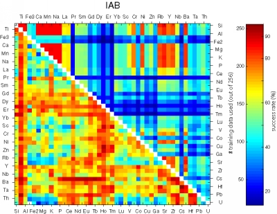
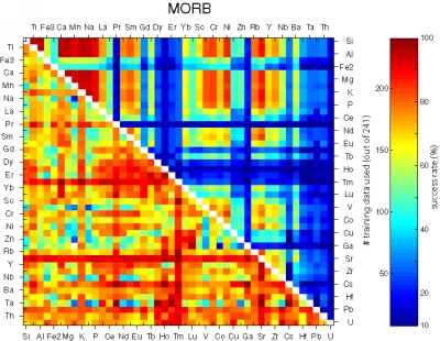
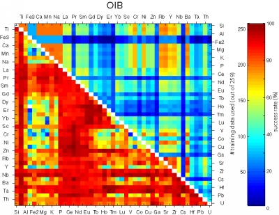
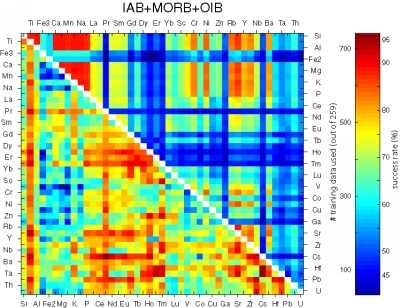
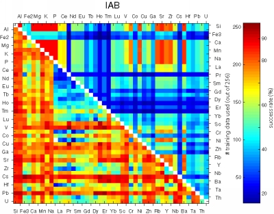
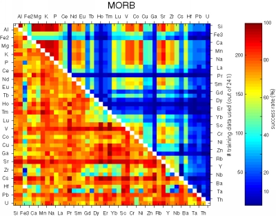
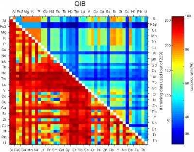
Figure 26:
Same as Figure 25, but for quadratic discriminant analysis.
|
|
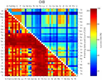
Figure 27:
Performance analysis of all possible ternary discriminant analyses
using TiO and other major element oxides.
|
|
Figure 28:
Same as Figure 27, but using quadratic discriminant analysis.
|
|
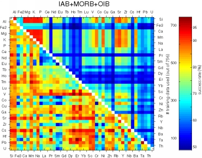
Figure 29:
Performance analysis of all possible ternary discriminant analyses
using Ti and two of 45 other elements.
|
|
Figure 30:
Same as Figure 29, but using quadratic discriminant analysis.
|
|
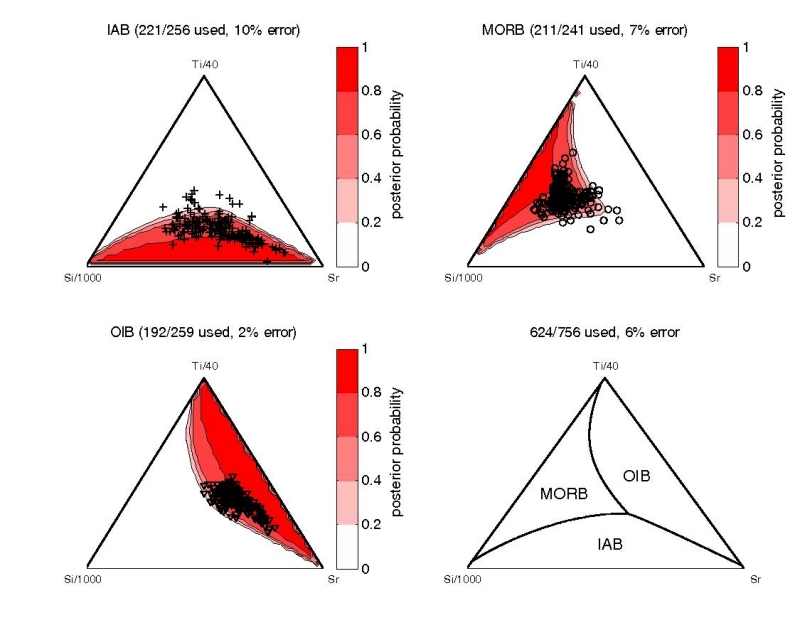
Figure 31:
The best ternary linear discriminant analysis, using Si, Ti, and Sr.
|
|
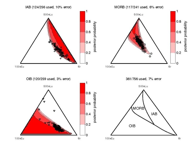
Figure 32:
Linear discriminant analysis using Eu, Lu, and Sr.
|
|
Figure 33:
The best performing linear discriminant analysis using only
incompatible elements (Ti, V and Sc).
|
|
Figure 34:
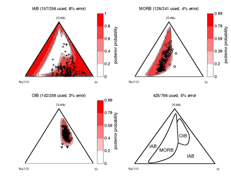
The best performing quadratic discriminant analysis, using Na, Nb and
Sr.
|
|
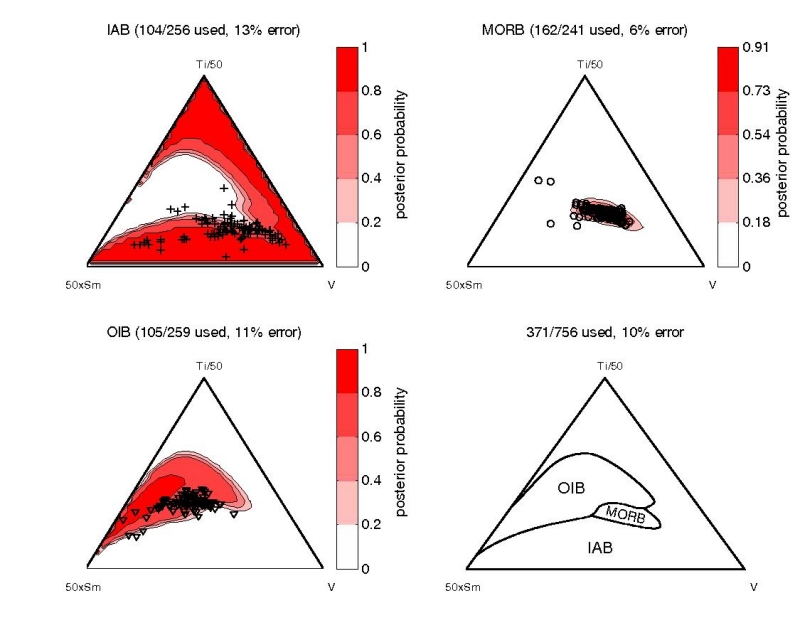
Figure 35:
The best performing quadratic discriminant analysis using only
incompatible elements (Ti, V and Sm).
|
|
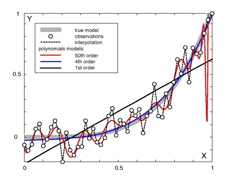
Figure 36:
Illustration of the bias-variance tradeoff in a regression context.
The thick gray line is the true model (Y = X ). The white circles
are 50 samples with random normal errors. The dashed line is the
interpolator, which is one of infinitely many functions that go
through all the datapoints and, thus, have zero bias. The solid black
line is a linear regression model, which has a large bias but small
variance. In this case, the fourth order polynomial (blue) is the best
predictor of future behavior. Although it has larger bias than the
50th order polynomial (red) and larger variance than the first order
polynomial (straight black line), it minimizes the mean squared error
(MSE = variance + bias
). The white circles
are 50 samples with random normal errors. The dashed line is the
interpolator, which is one of infinitely many functions that go
through all the datapoints and, thus, have zero bias. The solid black
line is a linear regression model, which has a large bias but small
variance. In this case, the fourth order polynomial (blue) is the best
predictor of future behavior. Although it has larger bias than the
50th order polynomial (red) and larger variance than the first order
polynomial (straight black line), it minimizes the mean squared error
(MSE = variance + bias ).
).
|
|
Figure 37:
The test data (116/182 used) plotted on various versions of the Ti-V
diagram with: a. the original decision boundaries of Shervais (1982),
drawn by eye; b. LDA on the logratio-plot, with anchor points 1-4
given in Table 6; c. QDA on the logratio-plot, d. the
same LDA as in subplot b., but this time mapped back to the
``traditional'' compositional data space; e. the QDA of subplot
c. mapped back to Ti-V space. An error analysis of these and
subsequent diagrams is given in Tables 5 and
7.
|
|
Figure 38:
The test data (89/182 used) plotted on the Ti-Zr diagram with: a. the
original decision boundaries of Pearce and Cann (1973); b-e as in
Figure 37.
|
|
Figure 39:
The test data (85/182 used) plotted on the Ti-Zr-Y diagram with:
a. the original decision boundaries of Pearce and Cann (1973); b-e as
in Figure 37.
|
|
Figure 40:
The test data (58/182 used) plotted on the Nb-Zr-Y diagram with: a.
the original decision boundaries of Meschede (1986); b-e as in Figure
37.
|
|
Figure 41:
The test data (36/182 used, but no MORBs!) plotted on the Th-Ta-Hf
diagram with: a. the original decision boundaries of Wood (1980); b-e
as in Figure 37.
|
|
Figure 42:
The test data (164/182 used) plotted on the Si-Ti-Sr LDA diagram
with: a. the decision boundaries and anchor points (see Table
6) in log-ratio space; b. the decision boundaries
mapped back to the simplex.
a. 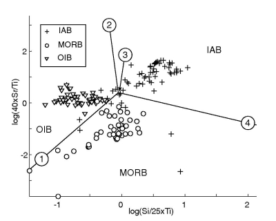
b. 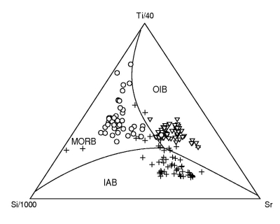
|
Figure 43:
The test data (103/182 used) plotted on the Eu-Lu-Sr LDA diagram; a
& b as in Figure 42.
a. 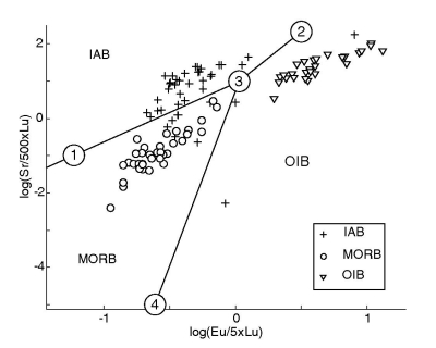
b. 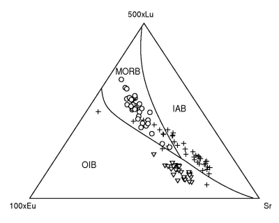
|
Figure 44:
The test data (72/182 used) plotted on the Ti-V-Sc LDA diagram; a &
b as in Figure 42.
a. 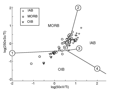
b. 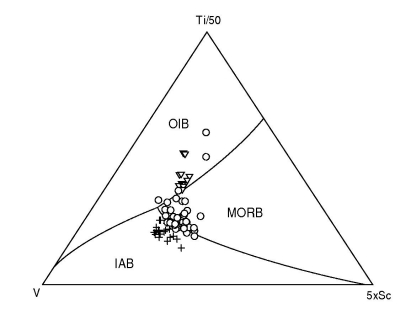
|
Figure 45:
The test data (61/182 used) plotted on the Na-Nb-Sr QDA diagram with:
a. the decision boundaries in log-ratio space; b. mapped back to
.
a. 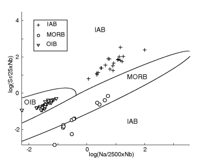
b. 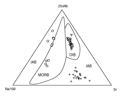
|
Figure 46:
The test data (85/182 used) plotted on the Ti-V-Sm QDA diagram; a &
b as in Figure 45.
a. 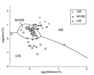
b. 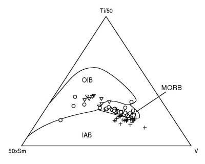
|
Next: About this document ...
Up: Tectonic discrimination diagrams revisited
Previous: List of Figures
Pieter Vermeesch
2005-11-21
 c.
c. 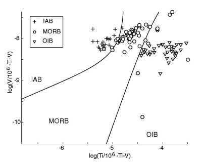 d.
d. 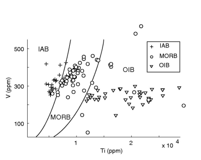 e.
e. 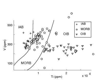
 c.
c. 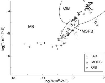 d.
d. 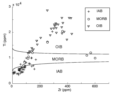 e.
e. 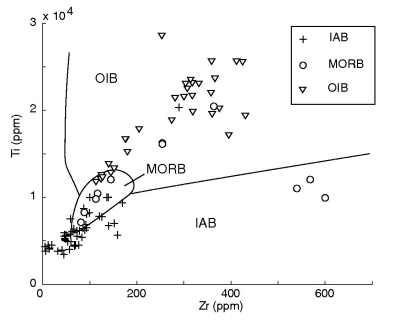
 c.
c. 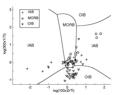 d.
d. 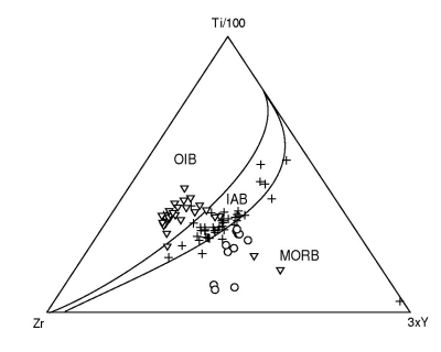 e.
e. 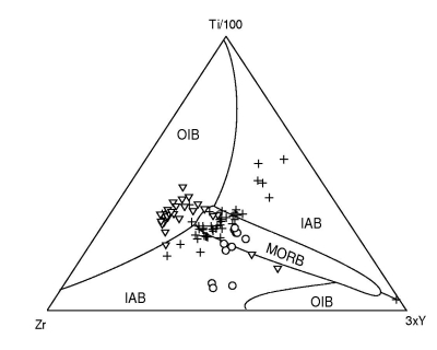
 c.
c. 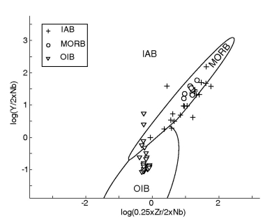 d.
d. 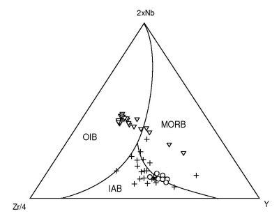 e.
e. 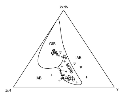
 c.
c. 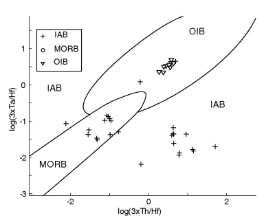 d.
d. 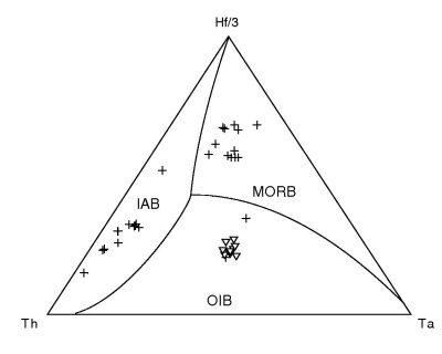 e.
e.