Consider a dataset of a large number of N-dimensional data X, which
belong to one of K classes. For example, X might be a set of
geochemical data (e.g., SiO![]() , Al
, Al![]() O
O![]() ,etc) from basaltic rocks
of K tectonic affinities (e.g., mid ocean ridge, ocean island, island
arc,...). We might ask ourselves which of these classes an unknown
sample x belongs to. This question is answered by Bayes' Rule:
the decision d is the class G (1
,etc) from basaltic rocks
of K tectonic affinities (e.g., mid ocean ridge, ocean island, island
arc,...). We might ask ourselves which of these classes an unknown
sample x belongs to. This question is answered by Bayes' Rule:
the decision d is the class G (1![]() G
G![]() K) that has the highest
posterior probability given the data x:
K) that has the highest
posterior probability given the data x:
where argmax stands for ``argument of the maximum'', i.e. when
f(k) reaches a maximum when k=d, then
![]() f(k) = d. This posterior distribution can be calculated according to
Bayes' Theorem:
f(k) = d. This posterior distribution can be calculated according to
Bayes' Theorem:
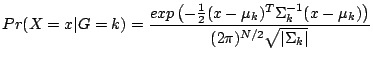
where Pr(X![]() G) is the probability density of the data in a
given class, and Pr(G) the prior probability of the class, which
we will consider uniformly distributed (i.e., Pr(G=1) = Pr(G=2) =
... = Pr(G=K) = 1/K) in this paper. Therefore, plugging Equation
2 into Equation 1 reduces Bayes' Rule
to a comparison of probability density estimates. We now make
the simplifying assumption of multivariate normality:
G) is the probability density of the data in a
given class, and Pr(G) the prior probability of the class, which
we will consider uniformly distributed (i.e., Pr(G=1) = Pr(G=2) =
... = Pr(G=K) = 1/K) in this paper. Therefore, plugging Equation
2 into Equation 1 reduces Bayes' Rule
to a comparison of probability density estimates. We now make
the simplifying assumption of multivariate normality:
Where ![]() and
and ![]() are the mean and covariance of the
k
are the mean and covariance of the
k![]() class and (x-
class and (x-![]() indicates the transpose of the matrix
(x-
indicates the transpose of the matrix
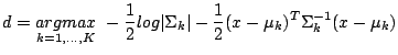
(x-![]() ). Using Equation 3, and taking
logarithms, Equation 1 becomes:
). Using Equation 3, and taking
logarithms, Equation 1 becomes:
Equation 4 is the basis for quadratic
discriminant analysis (QDA). Usually, ![]() and
and ![]() are not
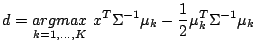
known, and must be estimated from the training data. If we make the
additional assumption that all the classes share the same covariance
structure (i.e.,
are not
known, and must be estimated from the training data. If we make the
additional assumption that all the classes share the same covariance
structure (i.e., ![]() =
= ![]()
![]() k), then Equation
1 simplifies to:
k), then Equation
1 simplifies to:
This is the basis of linear discriminant analysis (LDA), which
has some desirable properties. For example, because Equation
5 is linear in x, the decision boundaries between the
different classes are straight lines (Figure 8).
Furthermore, LDA can lead to a significant reduction in
dimensionality, in a similar way to principal component analysis
(PCA). PCA finds an orthogonal transformation B (i.e., a rotation)
that transforms the centered data (X) to orthogonality, so that the
elements of the vector BX are uncorrelated. B can be calculated by an
eigenvalue decomposition of the covariance matrix ![]() . The
eigenvectors are orthogonal linear combinations of the original
variables, and the eigenvalues give their variances. The first few
principal components generally account for most of the variability of
the data, constituting a significant reduction of dimensionality
(Figure 2).
. The
eigenvectors are orthogonal linear combinations of the original
variables, and the eigenvalues give their variances. The first few
principal components generally account for most of the variability of
the data, constituting a significant reduction of dimensionality
(Figure 2).
Like PCA, LDA also finds linear combinations of the original
variables. However, this time, we do not want to maximize the overall
variability, but find the orthogonal transformation Z = BX that
maximizes the between class variance S![]() relative to the
within class variance S
relative to the
within class variance S![]() , where S
, where S![]() is the variance of the class
means of Z, and S
is the variance of the class
means of Z, and S![]() is the pooled variance about the means (Figure
2).
is the pooled variance about the means (Figure
2).