Appendix B: details of the synthetic population generator.

Consider a specific value for M (the number of fractions), for example M=7. A population is generated by selecting an array of M-1 random numbers between zero and one, drawn from a uniform distribution (x$_i$, with i=1...6). This array is sorted and padded with a leading zero and a trailing one, becoming of size M+1.

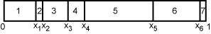
The difference between subsequent numbers in the array is a new array of size M (f$_j$, with j=1...7), in which each element represents a fraction of the total population. The population, when generated in this way, is automatically normalized to one.

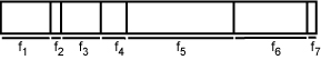
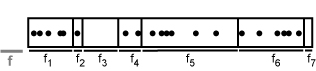
Random samples are generated by choosing k (for example 20) random numbers between zero and one, also from a uniform distribution. On the following figure, these numbers are marked by black dots. Each of the relevant fractions ("boxes") of the population is tested to see if the sample contains at least one number ("dot") that falls within it. On the next figure, the relevant fraction size f is marked by a gray bar. If at least one of the relevant fractions is empty, the test has failed. This is the case for our example, since the third box is empty and f$_3\geq$f. Note that fraction #7 is also empty, but this is irrelevant because f$_7<$f.

For each population, the ratio of the number of samples that failed the test to the total number of samples represents one estimate of p. This procedure is repeated for a large number of synthetically generated populations. The iterative process becomes of third order when a range of M values is evaluated (Figure 4).