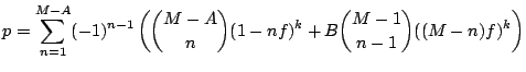
Consider a population that consists of M age fractions and define
relevant fractions to be those fractions that are greater than f. For
a given M (assuming M![]() 1/f), the worst-case scenario is that M-1
of the population fractions are of size f, and one fraction is of size
1-f(M-1). The probability p that at least one fraction
1/f), the worst-case scenario is that M-1
of the population fractions are of size f, and one fraction is of size
1-f(M-1). The probability p that at least one fraction ![]() f of the
population was missed is given by:
f of the
population was missed is given by:
This is a combinatoric expression where
![]() is the binomial
coefficient. Each term in the summation adds a correction to the
previous terms. Equation 2 is derived in Appendix A. For a
given number of relevant fractions m (m
is the binomial
coefficient. Each term in the summation adds a correction to the
previous terms. Equation 2 is derived in Appendix A. For a
given number of relevant fractions m (m![]() 1/f), a best-case
scenario can also be calculated (Appendix A):
1/f), a best-case
scenario can also be calculated (Appendix A):
Exploration of equations 2 and 3 over M and m, and
for different values of f and k, is shown in Figure 1. The
maximum number of (relevant) fractions for which Equations 2
and 3 are valid is 1/f. At larger values of M (or m), p is
kept constant. The shaded region on Figure 1a marks the
area where this is the case. One way to reduce the probability that
fractions ![]() f are missed when only k grains are dated is to
reduce the number of bins in the sample histogram. For example, if
k=60, f=0.05, and p=20%, then M
f are missed when only k grains are dated is to
reduce the number of bins in the sample histogram. For example, if
k=60, f=0.05, and p=20%, then M![]() =6 (Figure 1). A
detrital age-histogram that is constructed in this way conveys as much
information about the population as can be inferred from the sample
and is statistically "allowed" by p and f. However, it is less well
suited for showing the sample distribution. Therefore, such a
histogram should be used in conjunction with markers for the sample
data, or better still, a probability density plot
[6]. Such a combined plot carries an optimal amount
of information: the histogram represents the population with the
resolution that the data and the parameters p and f allow, while at
the same time, the probability density plot represents the data itself
and the uncertainties that are associated with it (Figure
2). M
=6 (Figure 1). A
detrital age-histogram that is constructed in this way conveys as much
information about the population as can be inferred from the sample
and is statistically "allowed" by p and f. However, it is less well
suited for showing the sample distribution. Therefore, such a
histogram should be used in conjunction with markers for the sample
data, or better still, a probability density plot
[6]. Such a combined plot carries an optimal amount
of information: the histogram represents the population with the
resolution that the data and the parameters p and f allow, while at
the same time, the probability density plot represents the data itself
and the uncertainties that are associated with it (Figure
2). M![]() usually is a rather small number, much smaller
than commonly used guidelines for the number of histogram bins such as
Sturges' rule [7,8]. Using M
usually is a rather small number, much smaller
than commonly used guidelines for the number of histogram bins such as
Sturges' rule [7,8]. Using M![]() will tend
to oversmooth the histogram, so although it theoretically is a viable
way to reduce the chance of missing significant fractions of the
population, there are better methods for dealing with datasets that
contain fewer than the optimal number of measurements. These methods
are discussed in the following paragraph and the Conclusions
section.
will tend
to oversmooth the histogram, so although it theoretically is a viable
way to reduce the chance of missing significant fractions of the
population, there are better methods for dealing with datasets that
contain fewer than the optimal number of measurements. These methods
are discussed in the following paragraph and the Conclusions
section.
Rather than reducing m, a much better way to reduce p is to increase k
or f. We now define p![]() as the maximum value of p, reached when
M=m=[1/f], where square brackets mark truncation to the nearest
integer. The equation for p
as the maximum value of p, reached when
M=m=[1/f], where square brackets mark truncation to the nearest
integer. The equation for p![]() is a special case of
(2):
is a special case of
(2):
Figure 3 shows the evolution of p![]() as a function of f
and k. Note the discrete "knee" in the p
as a function of f
and k. Note the discrete "knee" in the p![]() vs. f curve wherever
M = 1/f. Figure 3 can be used for a quick assessment of the
number of grains that are needed for a provenance study, and of the
risk of information loss that is caused by smaller samples. For
example, if 60 grains are dated, then
vs. f curve wherever
M = 1/f. Figure 3 can be used for a quick assessment of the
number of grains that are needed for a provenance study, and of the
risk of information loss that is caused by smaller samples. For
example, if 60 grains are dated, then ![]() =64%. Therefore, in
the worst-case scenario (which, at m=20, is a perfectly uniform
population) there is 64% chance that at least one fraction
=64%. Therefore, in
the worst-case scenario (which, at m=20, is a perfectly uniform
population) there is 64% chance that at least one fraction ![]() 0.05
of the population is missed. This is a dramatically different result
from the 5% probability suggested by Equation 1.
Furthermore, the actual fraction f
0.05
of the population is missed. This is a dramatically different result
from the 5% probability suggested by Equation 1.
Furthermore, the actual fraction f![]() that we can be sure not to
have missed with 95% certainty is not 0.05, but 0.085, as can be read
from Figure 3. Finally, and perhaps most importantly,
Figure 3 also shows that in order to be 95% confident that
no fraction
that we can be sure not to
have missed with 95% certainty is not 0.05, but 0.085, as can be read
from Figure 3. Finally, and perhaps most importantly,
Figure 3 also shows that in order to be 95% confident that
no fraction ![]() 0.05 was missed, at least k=117 grains must be
dated. Table 1 can be used to choose k, the number of grains required
to lower p and f to some desired limits. If fewer than this optimal
number of grains have been dated, Table 2 can be used to estimate the
actual levels of p and f that have been achieved with that k. The
same table also lists the value of
0.05 was missed, at least k=117 grains must be
dated. Table 1 can be used to choose k, the number of grains required
to lower p and f to some desired limits. If fewer than this optimal
number of grains have been dated, Table 2 can be used to estimate the
actual levels of p and f that have been achieved with that k. The
same table also lists the value of ![]() in the unlikely event
that the user prefers to reduce the resolution of the age histogram,
rather than to increase the desired p and/or f. Table 1 should be
used before embarking on a provenance study to determine how many
grains are needed. Alternatively, Table 2 can be used for the
interpretation of provenance data with less than the optimal number of
grains. For example, if only 30 grains have been dated, Table 2 says
that f
in the unlikely event
that the user prefers to reduce the resolution of the age histogram,
rather than to increase the desired p and/or f. Table 1 should be
used before embarking on a provenance study to determine how many
grains are needed. Alternatively, Table 2 can be used for the
interpretation of provenance data with less than the optimal number of
grains. For example, if only 30 grains have been dated, Table 2 says
that f![]() =0.15 is the smallest fraction not missed at a 95%
confidence level. Likewise, there is 20% chance of missing at least
one fraction representing
=0.15 is the smallest fraction not missed at a 95%
confidence level. Likewise, there is 20% chance of missing at least
one fraction representing ![]() 0.12 of the total population, and the
probability of missing at least one fraction
0.12 of the total population, and the
probability of missing at least one fraction ![]() 0.1 when 30 grains
were dated is 37%. Finally, to reduce the chance of missing at least
one fraction
0.1 when 30 grains
were dated is 37%. Finally, to reduce the chance of missing at least
one fraction ![]() 0.2 of the population to less than 10%, and still
only use 30 grains, the age-histogram cannot have more than
M
0.2 of the population to less than 10%, and still
only use 30 grains, the age-histogram cannot have more than
M![]() =5 bins. As an alternative to Figure 3, and to
Tables 1 and 2, an online web-form [9] is available for the
calculation of k, p
=5 bins. As an alternative to Figure 3, and to
Tables 1 and 2, an online web-form [9] is available for the
calculation of k, p![]() , f
, f![]() and M
and M![]() .
.
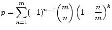
![$\displaystyle p_{max} = \sum_{n=1}^{[1/f]}(-1)^{n-1}
\binom{[1/f]}{n} (1-nf)^k$](img18.png)