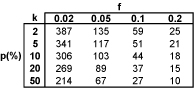
next up previous
Next: About this document ... Up: How many grains are Previous: Bibliography

Figures

Figure 1: Evolution of p$ _{max}$ with increasing number of population/sample fractions for a) a fixed number of measurements (k=60) and b) a fixed relevant fraction size (f=0.05). Solid lines represent worst- and dashed lines best-case scenarios. The shaded region on (a) marks the area where M$ \geq$1/f and p is kept constant at p$ _{max}$.
Image fig1a Image fig1b

Figure 2: As shown in Figure 1, at most M$ _{opt}$=6 bins are allowed in a sample histogram in order to reduce the chance that at least one fraction f$ \geq$0.05 is missed of a perfectly uniform population (worst-case scenario) to less than p=20%. The black dots represent the 60 samples. In histogram a, M=20$ \geq$M$ _{opt}$. In this particular example, three bins are empty, amounting to a total fraction 0.15 of the population. When the data are grouped into 20 bins, this occurs 64% of the time. In histogram b, M=M$ _{opt}$=6 and, for exactly the same sample, no fraction $ \geq$ 0.05 is missed. Only 20% of the histograms with 6 bins will have an empty fraction in their worst-case scenario, which corresponds to five fractions of size 0.05 and one of size 0.75. While using M$ _{opt}$ theoretically is a valid way to prevent relevant fractions of being missed, it will generally yield oversmoothed histograms and be of limited practical use. Instead, it is better to simply report f$ _{act}$ and/or p$ _{max}$ along with the data.
Image fig2a Image fig2b

Figure 3: Graphs that allow a quick assessment of the number of grains (k) needed to push the chance of missing at least one fraction $ \geq$f of a worst-case population below $ p_{max}$, a) as a function of the number of grains (k) and b) the number of (relevant) fractions (M) or their size (f).
Image fig3a Image fig3b

Table 1:
The adequate number of grains (k) as a function of the desired probability (p) of missing at least one fraction $ \geq$f of a worst-case population.
Image table1

Table 2
f$ _{act}$, p$ _{max}$ and M$ _{opt}$ as a function of k.
Image table2
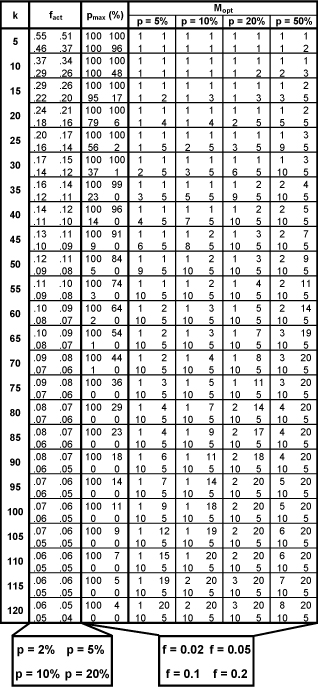
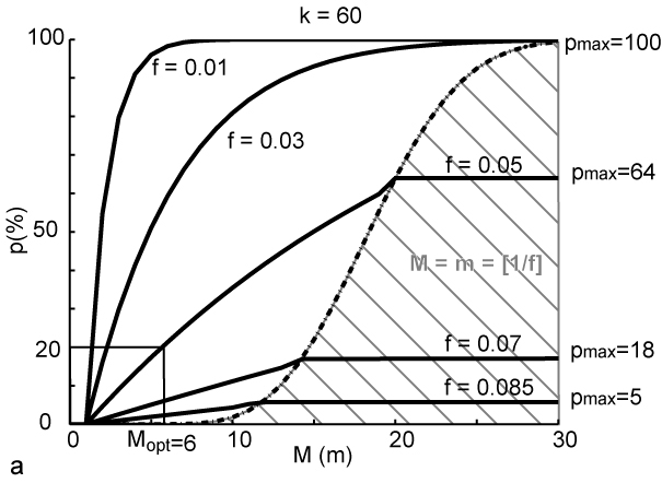
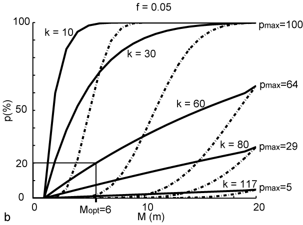
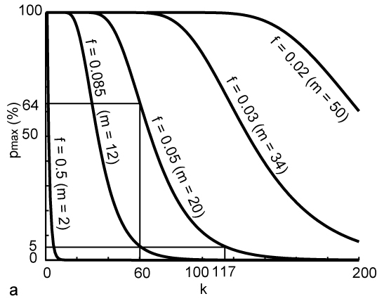
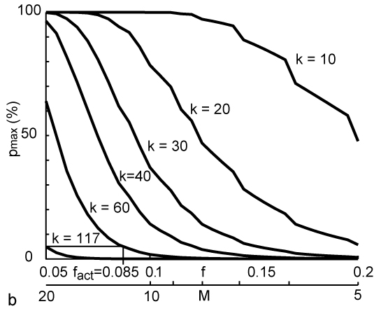
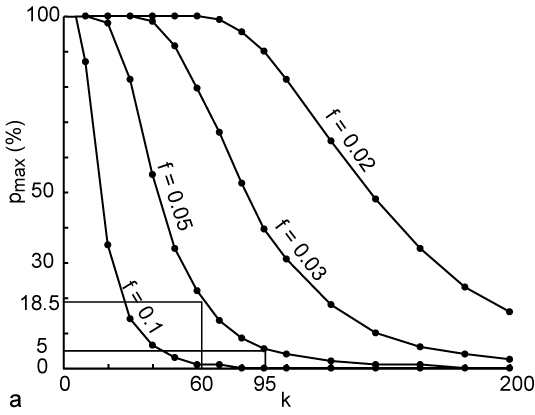
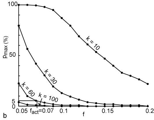
Given a specified number of grains (k), this Table shows f$ _{act}$ - the smallest population fraction that has not been missed with at least p% certainty - for four values of p; p$ _{max}$ - the maximum probability of missing at least one fraction $ \geq$f of a worst-case 
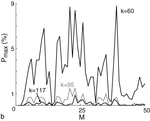
population - for four values of f; and M$ _{opt}$ - the largest number of bins that are less than p% likely to miss at least one fraction $ \geq$f of the worst-case population - for four values of f and p.

Figure 4: The random uniform numerical analogue to Figure 1, for k=60 and f=0.05. The solid black line gives the worst-case probability from Figure 1. The different symbols represent different levels of uniformity. The higher its "percentile", the closer a synthetic population is to a uniform distribution. For example, a "99 percentile" population is likely to be multimodal, while a "5 percentile" population would be nearly unimodal.
Image fig4

Figure 5: The numerical analogue to Figure 3, this plot allows a quick lookup of the maximum probability (p$ _{max}$) of missing at least one fraction $ \geq$f of a "95 percentile" synthetic population when k grains are dated.
Image fig5a Image fig5b

Figure 6: a) probability density plot of the Nubian Sandstone [11] and b) the result of numerical resampling experiments for different numbers of grains (k), for f=0.05.
Image fig6a Image fig6b

Figure 7: Same as Figure 6, but for the lunar impact spherules data [12].
Image fig7a Image fig7b


next up previous
Next: About this document ... Up: How many grains are Previous: Bibliography
Pieter Vermeesch 2004-05-19