In the previous section, we discussed the magnitude of the parentless
helium problem for small mineral inclusions. As will be demonstrated
later, it is possible to avoid this problem altogether (even for
relatively large inclusions) by dissolving the apatites and their
mineral inclusions in aggressive acids such as HF. However, this does
not solve a second problem, caused by the inhomogeneous U-Th
concentrations associated with mineral inclusions. ![]() -decay of
U, Th and their radioactive daughters is associated with energies of
4-8 MeV (Farley et al., 1996).
-decay of
U, Th and their radioactive daughters is associated with energies of
4-8 MeV (Farley et al., 1996). ![]() -particles with such high
energies travel on average 20
-particles with such high
energies travel on average 20 ![]() m in apatite before coming to rest.
Consider a spherical apatite with radius R and an
m in apatite before coming to rest.
Consider a spherical apatite with radius R and an ![]() -emitting
nuclide located at a radial distance X from its center. Let S be the
-emitting
nuclide located at a radial distance X from its center. Let S be the
![]() -stopping distance (e.g., 20
-stopping distance (e.g., 20 ![]() m).
m). ![]() -emitting
nuclides located at a distance R-S
-emitting
nuclides located at a distance R-S![]() X
X![]() R have a non-zero
probability of ejecting an
R have a non-zero
probability of ejecting an ![]() -particle outside the boundaries of
the apatite grain (Figure 2). For any given
spatial distribution of U and Th, it is possible to predict the
fraction (1-F
-particle outside the boundaries of
the apatite grain (Figure 2). For any given
spatial distribution of U and Th, it is possible to predict the
fraction (1-F![]() ) of radiogenic He lost by
) of radiogenic He lost by ![]() -ejection (Farley
et al., 1996; Meesters and Dunai, 2002; Hourigan et al. 2005). In
most cases, the U-Th distribution is not known and assumed to be
uniform. This assumption often constitutes the bulk of the analytical
(U-Th)/He age uncertainty. If significant He is produced by small
mineral inclusions, the assumption of uniform composition is violated.
We will address this problem mathematically for spherical grain
geometries. The physical dimension of the mineral inclusions will be
neglected, i.e. they will be considered point sources of
-ejection (Farley
et al., 1996; Meesters and Dunai, 2002; Hourigan et al. 2005). In
most cases, the U-Th distribution is not known and assumed to be
uniform. This assumption often constitutes the bulk of the analytical
(U-Th)/He age uncertainty. If significant He is produced by small
mineral inclusions, the assumption of uniform composition is violated.
We will address this problem mathematically for spherical grain
geometries. The physical dimension of the mineral inclusions will be
neglected, i.e. they will be considered point sources of
![]() -particles, making the He-retentivity of the inclusion itself
irrelevant.
-particles, making the He-retentivity of the inclusion itself
irrelevant.
If F![]() is the
is the ![]() -retention fraction of the apatite, and
F
-retention fraction of the apatite, and
F![]() is the fraction of
is the fraction of ![]() -particles that are ejected from
the inclusion but remain inside the apatite, then the total
-particles that are ejected from
the inclusion but remain inside the apatite, then the total
![]() -retention factor F
-retention factor F![]() can be defined as:
can be defined as:
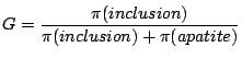
where G is the fraction of ![]() -decay activity (
-decay activity (![]() ) associated
with the mineral inclusion:
) associated
with the mineral inclusion:
with ![]() the decay constant and [n] the number of atoms or
moles of nuclide n (for n = 238, 235, 232 or 147). Note that equation
3 considers He-production to be a linear function of time,
which is a good approximation for relatively young samples (t
the decay constant and [n] the number of atoms or
moles of nuclide n (for n = 238, 235, 232 or 147). Note that equation
3 considers He-production to be a linear function of time,
which is a good approximation for relatively young samples (t ![]() 1/
1/
![]()
![]() n). Our goal is to derive the probability
distribution of F
n). Our goal is to derive the probability
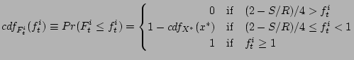
distribution of F![]() . To achieve this goal, we first compute the
cumulative distribution function (cdf) of the
. To achieve this goal, we first compute the
cumulative distribution function (cdf) of the ![]() -retention
factor F
-retention
factor F![]() :
:
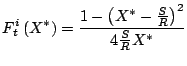
Where X![]() is the nondimensional radial distance X
is the nondimensional radial distance X![]() =X/R
corresponding to the
=X/R
corresponding to the ![]() -retention factor F
-retention factor F![]() . cdf
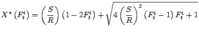
. cdf![]() can be computed because there exists a unique mapping between F
can be computed because there exists a unique mapping between F![]() and X
and X![]() (Figure 2), derived from equation 1 of
Farley et al. (1996):
(Figure 2), derived from equation 1 of
Farley et al. (1996):

|
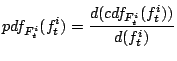
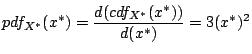
The probability density functions (pdfs) are then easily obtained by taking derivatives of the cdfs:
Using equations 8 and 9, we can calculate
![]() , the expected value of F
, the expected value of F![]() assuming that the
inclusions have a spatially uniform distribution. Here we use
``expected value'' in the statistical sense of the word, meaning the
average F
assuming that the
inclusions have a spatially uniform distribution. Here we use
``expected value'' in the statistical sense of the word, meaning the
average F![]() of many apatites containing a few inclusions, or the
average F
of many apatites containing a few inclusions, or the
average F![]() of a few apatites containing many inclusions. Thanks
to the mapping between F
of a few apatites containing many inclusions. Thanks
to the mapping between F![]() and X
and X![]() (equations 6
and 7 and Figure 2),
(equations 6
and 7 and Figure 2),
![]() can be calculated either by integrating over F
can be calculated either by integrating over F![]() or over X
or over X![]() .
Not surprisingly, both approaches yield the same result, which turns
out to be the analytical solution for F
.
Not surprisingly, both approaches yield the same result, which turns
out to be the analytical solution for F![]() under spherical geometry
calculated by Farley et al. (1996) for compositionally homogeneous
apatite:
under spherical geometry
calculated by Farley et al. (1996) for compositionally homogeneous
apatite:
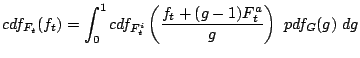
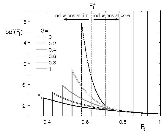
The probability distribution of F![]() (equation 1) can be
calculated for any G from the probability distribution for F
(equation 1) can be
calculated for any G from the probability distribution for F![]() (equation 8) and the expression for F
(equation 8) and the expression for F![]() given by
Farley et al. (1996) and equation 10 (Figure
3). Although G is not known in most cases, our ignorance
about G can be quantified by assigning a probability density function
pdf
given by
Farley et al. (1996) and equation 10 (Figure
3). Although G is not known in most cases, our ignorance
about G can be quantified by assigning a probability density function
pdf![]() to it. Again, to derive the probability distribution of
F
to it. Again, to derive the probability distribution of
F![]() , we must first define its cumulative density function
cdf
, we must first define its cumulative density function
cdf![]() :
:
|
with cdf
![]() as defined in equation 4, after
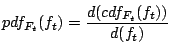
which pdf
as defined in equation 4, after
which pdf![]() is obtained by taking the derivative:
is obtained by taking the derivative:
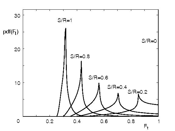
Figure 4 shows pdf![]() for a uniform pdf
for a uniform pdf![]() distribution and various S/R-values. The mode of the distribution is
always at F
distribution and various S/R-values. The mode of the distribution is
always at F![]() , with heavy tails, especially toward high
, with heavy tails, especially toward high
![]() -retentivities. If a ``normal''
-retentivities. If a ``normal'' ![]() -ejection correction
is made (F
-ejection correction
is made (F
![]() F
F![]() ) the most frequently measured age will
be accurate, but some other measurements will not. ``Undercorrected''
ages will generally be further removed from the true age than
``overcorrected'' ages. It would be relatively easy to compute F
) the most frequently measured age will
be accurate, but some other measurements will not. ``Undercorrected''
ages will generally be further removed from the true age than
``overcorrected'' ages. It would be relatively easy to compute F![]() -
and corresponding age-distributions for different, and possibly more
realistic pdf
-
and corresponding age-distributions for different, and possibly more
realistic pdf![]() s such as the logistic normal distribution. However,
such an exercise is of limited interest because in reality, pdf
s such as the logistic normal distribution. However,
such an exercise is of limited interest because in reality, pdf![]() is
not known. Nevertheless, the main features of Figures 3
and 4 are robust: the mean value of F
is
not known. Nevertheless, the main features of Figures 3
and 4 are robust: the mean value of F![]() equals
F
equals
F![]() and therefore the mean value of F
and therefore the mean value of F![]() is independent of
pdf
is independent of
pdf![]() . The distribution of F
. The distribution of F![]() has a sharp mode at F
has a sharp mode at F![]() , with
tails towards lower and higher values (Figure 4).
, with
tails towards lower and higher values (Figure 4).
|
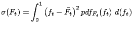
Given the probability distribution of F![]() (equation 12),
the standard deviation of F
(equation 12),
the standard deviation of F![]() can be calculated as:
can be calculated as:
Where ![]() =
= ![]() (equations 1 and
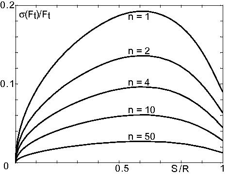
10). The relative spread (
(equations 1 and
10). The relative spread (![]() (
(![]() )/F
)/F![]() ) of the
single grain
) of the
single grain ![]() -retention factor F
-retention factor F![]() depends on the grain size
(Figure 5). For very small grains (S/R
depends on the grain size
(Figure 5). For very small grains (S/R ![]() 2),
the spread is zero because all
2),
the spread is zero because all ![]() He is ejected (F
He is ejected (F![]() = 0),
irrespective of the presence or absence of mineral inclusions. For
very large grains (S/R
= 0),
irrespective of the presence or absence of mineral inclusions. For
very large grains (S/R ![]() 0), the spread of F
0), the spread of F![]() is also zero,
because all
is also zero,
because all ![]() He stays within the apatite (F
He stays within the apatite (F![]()
![]() 1) and
the chance that a mineral inclusion is located within the outermost
fraction S/R of such an apatite is negligible. However, between these
two extremes, the spread of the
1) and
the chance that a mineral inclusion is located within the outermost
fraction S/R of such an apatite is negligible. However, between these
two extremes, the spread of the ![]() -retention factors is
non-zero, reaching a maximum at S/R
-retention factors is
non-zero, reaching a maximum at S/R ![]() 0.6, where
0.6, where
![]() /F
/F![]()
![]() 0.2. Please note that because the
F
0.2. Please note that because the
F![]() -distribution is not normally distributed (Figure
5), the 2
-distribution is not normally distributed (Figure
5), the 2![]() -value of 40% must not be
interpreted as the usual 95% confidence interval. However, by virtue
of the Central Limit Theorem, the average of n single-grain
measurements converges to a normal distribution with standard
deviation
-value of 40% must not be
interpreted as the usual 95% confidence interval. However, by virtue
of the Central Limit Theorem, the average of n single-grain
measurements converges to a normal distribution with standard
deviation ![]() (F
(F![]() )/
)/![]() . For example, the expected
2
. For example, the expected
2![]() -spread (corresponding to a 95% confidence interval) of
F
-spread (corresponding to a 95% confidence interval) of
F![]() -values for multi-grain packages containing n=10 grains each with
one inclusion, or single grains with n = 10 inclusions is less than
12%. If S/R = 1/3 (e.g., S = 20
-values for multi-grain packages containing n=10 grains each with
one inclusion, or single grains with n = 10 inclusions is less than
12%. If S/R = 1/3 (e.g., S = 20 ![]() m and R = 60
m and R = 60 ![]() m), then the
2
m), then the
2![]() confidence interval for F
confidence interval for F![]() is
is ![]() 10% (Figure
5). These estimates are conservative because they
assume that all the U and Th is contained in the mineral inclusions
and that the host apatite itself contains no U or Th. If this is not
the case, then the spread of the multi-grain ages will be smaller.
10% (Figure
5). These estimates are conservative because they
assume that all the U and Th is contained in the mineral inclusions
and that the host apatite itself contains no U or Th. If this is not
the case, then the spread of the multi-grain ages will be smaller.
|
<