Suppose we have N J-dimensional data points
X![]() ={x
={x![]() ,...,x
,...,x![]() ,...,x
,...,x![]() }, (1
}, (1![]() n
n![]() N) belonging
to one of K classes: Y
N) belonging
to one of K classes: Y![]() =c
=c![]()
![]() ...
...![]()
![]()
![]() ...
...![]()
![]() . For
example, X={X
. For
example, X={X![]() ,...,X
,...,X![]() ,...,X
,...,X![]() } might represent J
features (e.g., various major and trace element concentrations,
isotopic ratios, color, weight,...) measured in N samples of basalt.
c
} might represent J
features (e.g., various major and trace element concentrations,
isotopic ratios, color, weight,...) measured in N samples of basalt.
c![]() ,...,c
,...,c![]() might then be tectonic affinity, e.g., ``mid-ocean
ridge'', ``ocean island'', ``island arc'', ... . The basic idea
behind classification and regression trees (CART) is to approximate
the parameter space by a piecewise constant function, in other words,
to partition X into M disjoint regions
{R
might then be tectonic affinity, e.g., ``mid-ocean
ridge'', ``ocean island'', ``island arc'', ... . The basic idea
behind classification and regression trees (CART) is to approximate
the parameter space by a piecewise constant function, in other words,
to partition X into M disjoint regions
{R![]() ,...,R
,...,R![]() ,...,R
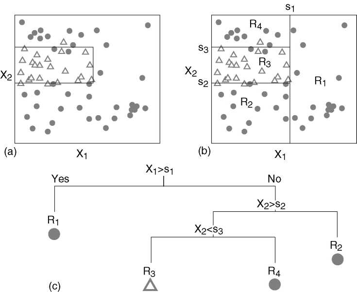
,...,R![]() }. An example of such a partition is given
in Figure 1.a. Because it is impossible to describe
all possible partitions of the feature space, we restrict ourselves to
a small subset of possible solutions, the recursive binary partitions
(Figure 1.b). Surprising as it may seem,
considering the crudeness of this approximation, trees are one of the
most powerful and popular data mining techniques in existence. One of
the reasons for this is that besides assuring computational
feasibility, the recursive partitioning technique described next also
allows the representation of the multi-dimensional decision-space as a
two dimensional tree graph (Figure 1.c). Although
building a tree might seem complicated, this is not important to the
user, because it only has to be done once, after which using a
classification tree for data interpretation is extremely simple.
}. An example of such a partition is given
in Figure 1.a. Because it is impossible to describe
all possible partitions of the feature space, we restrict ourselves to
a small subset of possible solutions, the recursive binary partitions
(Figure 1.b). Surprising as it may seem,
considering the crudeness of this approximation, trees are one of the
most powerful and popular data mining techniques in existence. One of
the reasons for this is that besides assuring computational
feasibility, the recursive partitioning technique described next also
allows the representation of the multi-dimensional decision-space as a
two dimensional tree graph (Figure 1.c). Although
building a tree might seem complicated, this is not important to the
user, because it only has to be done once, after which using a
classification tree for data interpretation is extremely simple.
|